Aligning Spatial Glycomics and IHC images#
Author:Andrew Causer
This notebook is a tutorial of how to use goatpy to align IHC images with spatial glycomics data. For more infomation on image alignment with goatpy please visit the Getting Started page.
Similar to using a H&E image, IHC images can be aligned to Glycomics data with goatpy using either a manual or automatic method.
[1]:
import goatpy as gp
import spatialdata_plot
import matplotlib.pyplot as plt
import scanpy as sc
import pandas as pd
import squidpy as sq
from napari_spatialdata import Interactive
Manual Alignment#
Manual alignment involves the use of SpatialData-Napari. First we need to contruct two SpatialData objects using goatpy:
Spatial Glycomics Object (MALDI-MSI)
Imaging Data Object (IHC)
Lets do this below:
[2]:
## Create MALDI-MSI SpatialData object
maldi_sd = gp.glyco_spatialdata(imzml_path="./Documents/IHC_test_data/ad_dm_sa_deriv_19pm0001_0204002_reduced_peakonly.imzML")

## Create IHC SpatialData object
ihc_sd = gp.ihc_spatialdata("./Documents/IHC_test_data/DM_22.05.26_Image_2_19PM0001_RedGrnChannel.tif")
Loaded image with shape: (1341, 1508, 3)
Successfully generated SpatialData object
We can visualise the data structure of these two objects:
[3]:
maldi_sd
[3]:
SpatialData object
├── Points
│     └── 'centroids': DataFrame with shape: (<Delayed>, 112) (2D points)
├── Shapes
│     └── 'pixels': GeoDataFrame shape: (117948, 2) (2D shapes)
└── Tables
      └── 'maldi_adata': AnnData (117948, 108)
with coordinate systems:
    ▸ 'global', with elements:
        centroids (Points), pixels (Shapes)
[4]:
ihc_sd
[4]:
SpatialData object
└── Images
      └── 'ihc_image': DataArray[cyx] (3, 1341, 1508)
with coordinate systems:
    ▸ 'global', with elements:
        ihc_image (Images)
Following the same method as H&E manual alignment we must generate a psuedo-image for our MALDI-MSI data:
[5]:
maldi_sd = gp.Add_Pseudo_Image(maldi_sd, "MPI", tables = "maldi_adata", library_id = "Spatial", is_continous=True, cmap = "viridis",img_upscaling=2)
INFO Transposing `data` of type: <class 'dask.array.core.Array'> to ('c', 'y', 'x').
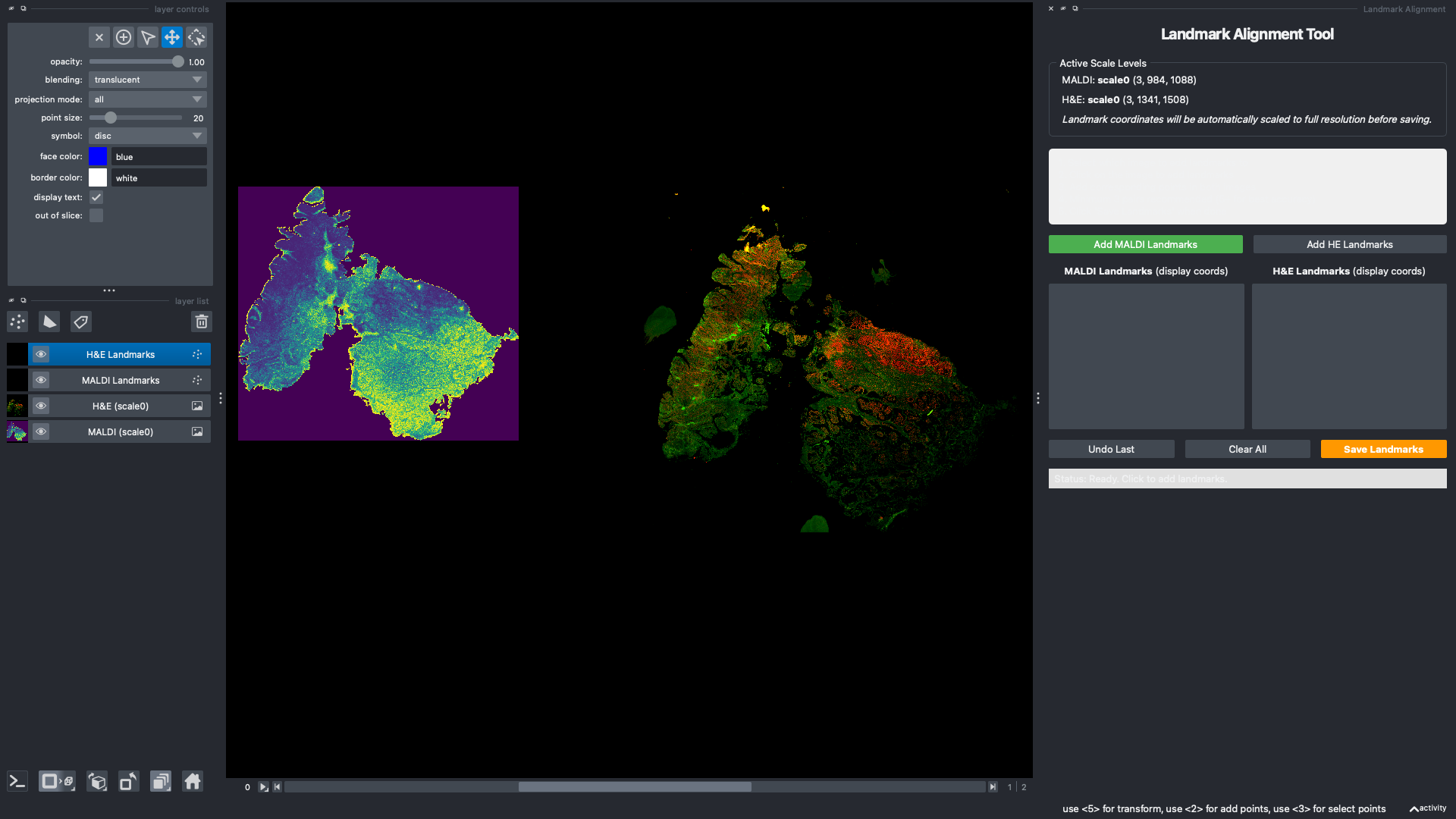
Now we can run goatpy’s manual alignment GUI to select corresponding landmarks on the pseudo-MSI and IHC image. Below is a screenshot showing the layout of the single window GUI:
[ ]:
viewer, widget = gp.launch_landmark_gui(maldi_sd, ihc_sd, split_view=False, he_image_key = "ihc_image")
The below section of code is for reproducability. These are the location of 4 landmarks on the MALDI-MSI and IHC coordinate system, respectively.
[6]:
from spatialdata.models import PointsModel
import pandas as pd

maldi_align_points = pd.DataFrame({
    "x": [56.691345,172.349422,577.152689,997.829025,],
    "y": [483.286246,166.483689,322.370662,597.166866]
})

ihc_align_points = pd.DataFrame({
    "x": [129.072657,318.347858,834.765384,1318.743398],
    "y": [669.121976,267.204264,503.214083,870.946993]
})

maldi_sd["maldi_landmarks"] = PointsModel.parse(maldi_align_points)
ihc_sd["ihc_landmarks"] = PointsModel.parse(ihc_align_points)
Following the selection of these landmarks we can run the alignment function.
NOTE: Make sure the correct image keys are used if changed between H&E and IHC images.
[7]:
aligned = gp.align_image_using_landmarks(maldi_sd, ihc_sd, he_image_key = "ihc_image", he_landmark_key = "ihc_landmarks")
[8]:
aligned.pl.render_images("ihc_image") \
       .pl.render_shapes("pixels", color="MPI", size =50) \
       .pl.show("aligned")
INFO     Using 'datashader' backend with 'None' as reduction method to speed up plotting. Depending on the
         reduction method, the value range of the plot might change. Set method to 'matplotlib' to disable this
         behaviour.
INFO     Using the datashader reduction "mean". "max" will give an output very close to the matplotlib result.
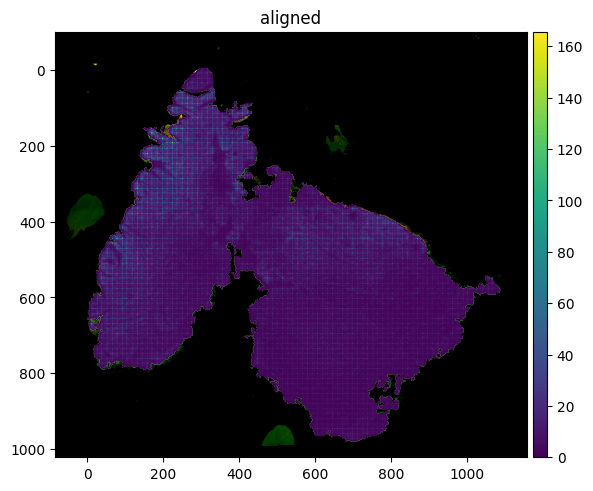
From the figure above we can see the alignment has worked well.
Automatic Alignment#
Similar to H&E, we can also run automatic alignment with the IHC image. Lets run this below, providing the .imzML, IHC image and peaks list file path.
[9]:
sdata = gp.load_and_align(imzml_path="./Documents/IHC_test_data/ad_dm_sa_deriv_19pm0001_0204002_reduced_peakonly.imzML",
               ihc_path="./Documents/IHC_test_data/DM_22.05.26_Image_2_19PM0001_RedGrnChannel.tif",
               peaks_path="./Documents/IHC_test_data/Sample 19M0001 glycan list.csv")
[0.23GB] Loading peaks ...
[0.24GB]   174 peaks
[0.24GB]   IHC pixel size from ImageJ TIFF tags (ResolutionUnit=1, unit=µm): 7.8000 um/px  (XResolution=0.128205 px/µm)
[0.24GB]   IHC native pixel size: 7.8000 um/px
[0.29GB]   MALDI pixel size from imzML metadata: 20.0 um/px
[0.25GB]   Validated: ref thumbnail (588x523 px) >= MALDI (544x492 px)
[0.25GB]   maldi_pixel_um=20.0  ref_pixel_um=7.8000
[0.25GB] Computing MALDI crop offsets ...
[0.30GB]   Crop: row=0, col=0
[0.70GB] Loading 174 ion images (chunk=10) with 0.1 Da tolerance per peak ...
[0.44GB]   Peaks 1-10 / 174
[0.44GB]   Peaks 11-20 / 174
[0.45GB]   Peaks 21-30 / 174
[0.46GB]   Peaks 31-40 / 174
[0.44GB]   Peaks 41-50 / 174
[0.43GB]   Peaks 51-60 / 174
[0.44GB]   Peaks 61-70 / 174
[0.43GB]   Peaks 71-80 / 174
[0.43GB]   Peaks 81-90 / 174
[0.43GB]   Peaks 91-100 / 174
[0.46GB]   Peaks 101-110 / 174
[0.43GB]   Peaks 111-120 / 174
[0.46GB]   Peaks 121-130 / 174
[0.32GB]   Peaks 131-140 / 174
[0.32GB]   Peaks 141-150 / 174
[0.29GB]   Peaks 151-160 / 174
[0.31GB]   Peaks 161-170 / 174
[0.32GB]   Peaks 171-174 / 174
[0.35GB]   spectra_all: (492, 544, 174)  (186 MB)
[0.35GB] Preparing MALDI template ...
[0.35GB]   MALDI grayscale: (492, 544)  mean=0.192
[0.74GB] Loading IHC at 20.0 um/px ...
[0.74GB]   Loading IHC: ./Documents/IHC_test_data/DM_22.05.26_Image_2_19PM0001_RedGrnChannel.tif
[0.74GB]   Raw array shape: (1341, 1508, 3)  dtype=uint8  axes='YXS'
[0.74GB]   Normalised to (C,H,W): (3, 1341, 1508)
[0.74GB]   Channel names: ['CF_405', 'CF_488', 'CF_561']
[0.74GB]   Auto-selected registration channel 1 ('CF_488', mean=13.4)
[0.74GB]   Resizing: (1341, 1508) -> (523, 588)  scale=0.3900  (7.800 -> 20.000 um/px)
[0.76GB]   IHC at reg resolution: (3, 523, 588)  20.000 um/px  (0.9 MB)
[0.76GB] Preparing IHC registration image ...
[0.76GB]   IHC grayscale: (523, 588)  mean=0.053  (invert=False)
[0.76GB] Running registration ...
[0.76GB]   Coarse: 24 rotations (0-360 step 15) ...
[0.77GB]       0.0  score=0.5745
[0.78GB]      15.0  score=0.4680
[0.80GB]      30.0  score=0.4026
[0.81GB]      45.0  score=0.3938
[0.82GB]      60.0  score=0.3977
[0.83GB]      75.0  score=0.3542
[0.83GB]      90.0  score=0.3256
[0.83GB]     105.0  score=0.3269
[0.84GB]     120.0  score=0.3869
[0.85GB]     135.0  score=0.3855
[0.86GB]     150.0  score=0.3698
[0.86GB]     165.0  score=0.3843
[0.86GB]     180.0  score=0.3616
[0.87GB]     195.0  score=0.3575
[0.87GB]     210.0  score=0.3397
[0.88GB]     225.0  score=0.3499
[0.88GB]     240.0  score=0.3742
[0.88GB]     255.0  score=0.3260
[0.88GB]     270.0  score=0.2170
[0.88GB]     285.0  score=0.2460
[0.88GB]     300.0  score=0.2588
[0.88GB]     315.0  score=0.2950
[0.89GB]     330.0  score=0.3452
[0.89GB]     345.0  score=0.4896
[0.89GB]   Best coarse: 0.0  score=0.5745
[0.89GB]   Fine: 10 rotations (+-5.0 step 1.0) ...
[0.89GB]      -5.0  score=0.6059
[0.89GB]      -4.0  score=0.6262
[0.89GB]      -3.0  score=0.6384
[0.89GB]      -2.0  score=0.6277
[0.89GB]      -1.0  score=0.6122
[0.89GB]       1.0  score=0.5813
[0.89GB]       2.0  score=0.5682
[0.89GB]       3.0  score=0.5584
[0.89GB]       4.0  score=0.5481
[0.89GB]       5.0  score=0.5374
[0.89GB]   Final: -3.0  score=0.6384  offset=(123, 116)
[0.89GB] Building output canvas ...
[0.89GB]   IHC canvas (cv2): 764x703  channels=3  pr=75, pc=75  rotation=-3.0
[0.89GB] Building SpatialData ...
[0.99GB]   H&E upscaled 10x: 7640x7030  (161 MB)
[1.42GB]   IHC upscaled 10x: (3, 7030, 7640)  (161 MB)
[1.41GB]   IHC image stored: channels=['CF_405', 'CF_488', 'CF_561']
[1.43GB]   Transform stored: mode=ihc  rotation=-3.0  ref_reg_size=[523, 588]  canvas_placement=[75, 75]
[1.43GB] Done.
[10]:
sdata
[10]:
SpatialData object
├── Images
│     └── 'ihc_image': DataArray[cyx] (3, 7030, 7640)
├── Points
│     └── 'centroids': DataFrame with shape: (<Delayed>, 3) (2D points)
├── Shapes
│     └── 'pixels': GeoDataFrame shape: (267648, 2) (2D shapes)
└── Tables
      └── 'maldi_adata': AnnData (267648, 174)
with coordinate systems:
    ▸ 'global', with elements:
        ihc_image (Images), centroids (Points), pixels (Shapes)
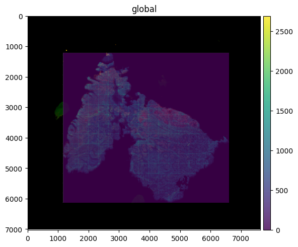
[11]:
sdata.pl.render_images("ihc_image") \
     .pl.render_shapes("pixels", color="MPI", fill_alpha = 0.8) \
     .pl.show()
INFO     Rasterizing image for faster rendering.
INFO     Using 'datashader' backend with 'None' as reduction method to speed up plotting. Depending on the
         reduction method, the value range of the plot might change. Set method to 'matplotlib' to disable this
         behaviour.
INFO     Using the datashader reduction "mean". "max" will give an output very close to the matplotlib result.
Spatially Informed Clustering (GraphPCA)#
goatpy has also integrated the use of GraphPCA spatial clustering. Spatial infomation can often improve clustering compared to non-spatial methods (i.e. leiden).
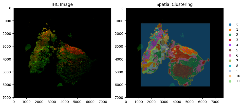
Below we will run spatial_clustering and visualise the results overlayed with the IHC image:
[12]:
sdata = gp.graphpca_spatialdata(sdata, tables= "maldi_adata",
    library_id= 'spatial',
    n_components = 50,
    n_neighbors = 15,
    alpha = 0.5)

sdata = gp.get_kmean_clusters(sdata, tables= "maldi_adata",n_clusters = 12)
[13]:
fig, axes = plt.subplots(1, 2, figsize=(10, 5))

sdata.pl.render_images("ihc_image") \
     .pl.show(ax=axes[0], title="IHC Image")

sdata.pl.render_images("ihc_image") \
     .pl.render_shapes("pixels",size = 3,fill_alpha = 0.5,color="GPCA_clusters") \
     .pl.show(ax=axes[1], title="Spatial Clustering")

plt.tight_layout()
plt.show()
INFO     Rasterizing image for faster rendering.
INFO     Rasterizing image for faster rendering.
INFO     Using 'datashader' backend with 'None' as reduction method to speed up plotting. Depending on the
         reduction method, the value range of the plot might change. Set method to 'matplotlib' to disable this
         behaviour.
Align Additional Image Layers#
This process can be repated to align additional image layers such as both IHC and H&E. Once aligning the first image to the MALDI-MSI (with either the manual or automatic alignment method), we can use the manual landmark based alignment to align any additional images.
Below we will align the H&E image to the aligned IHC data object:
[14]:
he_sd = gp.he_spatialdata( "./Documents/IHC_test_data/HnE_Image_64.vsi - 40x_BF_01.jpg")

viewer, widget = gp.launch_landmark_gui(sdata, he_sd, split_view=False, maldi_image_key = "ihc_image", he_image_key = "he_image")
./goatpy/goatpy/he_image.py:30: UserWarning: sopa.io.wsi failed! Try running `pip install openslide`. Falling back to PIL method.
  warnings.warn(f"sopa.io.wsi failed! Try running `pip install {backend}`. Falling back to PIL method. ")
Available MALDI scale levels:
  scale0: (3, 7030, 7640)
Available H&E scale levels:
  scale0: (3, 8076, 8899)

No maldi_scale_level specified — defaulting to 'scale0'.

Launching GUI with MALDI=scale0, H&E=scale0
[LandmarkGUI] MALDI display level=scale0, scale_factor=1.000  |  H&E display level=scale0, scale_factor=1.000
INFO: Saved 4 landmark pairs (scaled to full resolution)
[15]:
maldi_align_points = pd.DataFrame({
    "x": [2022.968467,3141.007734,5635.143076,3378.290817],
    "y": [2015.704049,2654.583630,3650.106883,5073.061192]
})

he_align_points = pd.DataFrame({
    "x": [1424.905810,3255.734239,7221.517791,3632.379621],
    "y": [1343.220173,2316.813290,4056.500643,6329.981808]
})

sdata["maldi_landmarks"] = PointsModel.parse(maldi_align_points)
he_sd["he_landmarks"] = PointsModel.parse(he_align_points)
[16]:
aligned = gp.align_image_using_landmarks(sdata, he_sd, maldi_image_key = "ihc_image", he_image_key = "he_image", he_landmark_key = "he_landmarks")
[17]:
aligned
[17]:
SpatialData object
├── Images
│     ├── 'he_image': DataArray[cyx] (3, 8076, 8899)
│     └── 'ihc_image': DataArray[cyx] (3, 7030, 7640)
├── Points
│     ├── 'centroids': DataFrame with shape: (<Delayed>, 3) (2D points)
│     ├── 'he_landmarks': DataFrame with shape: (<Delayed>, 2) (2D points)
│     └── 'maldi_landmarks': DataFrame with shape: (<Delayed>, 2) (2D points)
├── Shapes
│     └── 'pixels': GeoDataFrame shape: (267648, 2) (2D shapes)
└── Tables
      └── 'maldi_adata': AnnData (267648, 174)
with coordinate systems:
    ▸ 'aligned', with elements:
        he_image (Images), ihc_image (Images), centroids (Points), he_landmarks (Points), maldi_landmarks (Points), pixels (Shapes)
    ▸ 'global', with elements:
        he_image (Images), ihc_image (Images), centroids (Points), he_landmarks (Points), maldi_landmarks (Points), pixels (Shapes)
[18]:
fig, axes = plt.subplots(1, 2, figsize=(10, 5))

aligned.pl.render_images("ihc_image") \
     .pl.render_shapes("pixels",size = 3,fill_alpha = 0.3,color="GPCA_clusters") \
     .pl.show("aligned", ax=axes[0], title="IHC + Spatial Clustering")

aligned.pl.render_images("he_image") \
     .pl.render_shapes("pixels",size = 3,fill_alpha = 0.3,color="GPCA_clusters") \
     .pl.show("aligned", ax=axes[1], title="H&E + Spatial Clustering")

plt.tight_layout()
plt.show()
INFO     Rasterizing image for faster rendering.
INFO     Using 'datashader' backend with 'None' as reduction method to speed up plotting. Depending on the
         reduction method, the value range of the plot might change. Set method to 'matplotlib' to disable this
         behaviour.
INFO     Rasterizing image for faster rendering.
INFO     Using 'datashader' backend with 'None' as reduction method to speed up plotting. Depending on the
         reduction method, the value range of the plot might change. Set method to 'matplotlib' to disable this
         behaviour.

This object can now be used to run downstream analysis using goatpy or any other package:
Tutorial Session Info#
[19]:
from session_info import show
show()
[19]:
Click to view session information
-----
anndata             0.11.4
debugpy             1.8.20
geopandas           1.1.2
goatpy              0.1.0
ipykernel           6.31.0
matplotlib          3.10.8
napari              0.6.6
napari_spatialdata  0.6.0
pandas              2.3.3
scanpy              1.11.5
session_info        v1.0.1
spatialdata         0.5.0
spatialdata_plot    0.2.12
squidpy             1.6.5
-----
Click to view modules imported as dependencies
81d243bd2c585b0f4821__mypyc NA
PIL                         12.1.1
PyQt5                       NA
ac51d50a4f4b6d748b8c__mypyc NA
annotated_types             0.7.0
app_model                   0.4.0
appdirs                     1.4.4
appnope                     0.1.4
asciitree                   NA
asttokens                   NA
attr                        25.4.0
attrs                       25.4.0
babel                       2.18.0
backports                   NA
bermuda                     NA
cachey                      0.2.1
certifi                     2026.02.25
charset_normalizer          3.4.5
click                       8.3.1
cloudpickle                 3.1.2
colorama                    0.4.6
comm                        0.2.3
cv2                         4.13.0
cycler                      0.12.1
cython_runtime              NA
dask                        2024.11.2
dask_image                  NA
datashader                  0.18.2
dateutil                    2.9.0.post0
decorator                   5.2.1
distributed                 2024.11.2
docrep                      0.3.2
docstring_parser            NA
exceptiongroup              1.3.1
executing                   2.2.1
flexcache                   0.3
flexparser                  0.4
fontTools                   4.61.1
fsspec                      2026.2.0
h5py                        3.16.0
heapdict                    NA
hsluv                       5.0.4
idna                        3.11
igraph                      1.0.0
imagecodecs                 2025.3.30
imageio                     2.37.2
importlib_metadata          NA
in_n_out                    0.2.1
jaraco                      NA
jedi                        0.19.2
jinja2                      3.1.6
joblib                      1.5.3
jsonschema                  4.26.0
jsonschema_specifications   NA
kiwisolver                  1.4.9
lazy_loader                 0.5
legacy_api_wrap             NA
leidenalg                   0.11.0
llvmlite                    0.46.0
locket                      NA
loguru                      0.7.3
lxml                        6.1.1
magicgui                    0.10.1
markupsafe                  3.0.3
matplotlib_inline           0.2.1
matplotlib_scalebar         0.9.0
metaspace                   2.0.9
metaspace_converter         NA
more_itertools              10.8.0
mpl_toolkits                NA
msgpack                     1.1.2
multipledispatch            0.6.0
multiscale_spatial_image    2.0.3
napari_builtins             0.6.6
napari_plugin_engine        0.2.1
natsort                     8.4.0
networkx                    3.4.2
npe2                        0.8.1
numba                       0.64.0
numcodecs                   0.13.1
numpy                       2.2.6
numpydoc                    1.10.0
ome_zarr                    NA
openslide                   1.4.3
openslide_bin               4.0.0.12
packaging                   26.0
parso                       0.8.6
patsy                       1.0.2
pexpect                     4.9.0
pims                        0.7
pint                        0.24.4
pkg_resources               NA
platformdirs                4.9.4
plotly                      6.6.0
prompt_toolkit              3.0.52
psutil                      7.2.2
psygnal                     0.15.1
ptyprocess                  0.7.0
pure_eval                   0.2.3
pyarrow                     21.0.0
pyct                        0.6.0
pydantic                    2.12.5
pydantic_compat             0.1.2
pydantic_core               2.41.5
pydantic_extra_types        2.11.0
pydev_ipython               NA
pydevconsole                NA
pydevd                      3.2.3
pydevd_file_utils           NA
pydevd_plugins              NA
pydevd_tracing              NA
pygments                    2.19.2
pyimzml                     1.5.5
pyparsing                   3.3.2
pyproj                      3.7.1
pyqtgraph                   0.14.0
pytz                        2026.1.post1
qtpy                        2.4.3
referencing                 NA
requests                    2.32.5
rich                        NA
rpds                        NA
scipy                       1.15.3
seaborn                     0.13.2
shapely                     2.1.2
sip                         NA
six                         1.17.0
skimage                     0.25.2
sklearn                     1.7.2
slicerator                  1.1.0
sopa                        2.1.11
sortedcontainers            2.4.0
spatial_image               1.2.3
sphinxcontrib               NA
stack_data                  0.6.3
statsmodels                 0.14.6
superqt                     0.8.0
tblib                       3.2.2
texttable                   1.7.0
threadpoolctl               3.6.0
tifffile                    2025.5.10
tlz                         1.1.0
toolz                       1.1.0
torch                       2.10.0
torchgen                    NA
tornado                     6.5.4
tqdm                        4.67.3
traitlets                   5.14.3
triangle                    20250106
typing_extensions           NA
typing_inspection           NA
urllib3                     2.6.3
validators                  0.35.0
vispy                       0.15.2
vscode                      NA
wcwidth                     0.6.0
wrapt                       2.1.2
xarray                      2025.6.1
xarray_dataclass            3.0.0
xarray_schema               0.0.3
xrspatial                   0.5.3
yaml                        6.0.3
zarr                        2.18.3
zict                        3.0.0
zipp                        NA
zmq                         27.1.0
zoneinfo                    NA
-----
IPython             8.38.0
jupyter_client      8.8.0
jupyter_core        5.9.1
-----
Python 3.10.19 | packaged by conda-forge | (main, Oct 22 2025, 22:46:49) [Clang 19.1.7 ]
macOS-26.3.1-arm64-arm-64bit
-----
Session information updated at 2026-05-30 19:32