Multi-Sample goatpy Analysis Tutorial#
Author:Andrew Causer
This notebook is a tutorial of how to use goatpy for analysing multiple Glycomics data samples. For an a more general introduction on how to use goatpy please visit `Getting Started with goatpy <>`__ or the goatpy Github site.
Loading Data#
First we will load all required packages and run automatic alignment:
[1]:
import goatpy as gp
from spatialdata import read_zarr
import spatialdata_plot
import matplotlib.pyplot as plt
import scanpy as sc
import squidpy as sq
import pandas as pd
import napari
import numpy as np
from napari_spatialdata import Interactive
After importing packages we can load our two samples:
[2]:
b19 = gp.load_and_align(imzml_path = "./Documents/test_data/breast_cancer_concr_0019/concr_tnbc_0019-s1-total_ion_count.imzML",
                        peaks_path = "./Documents/test_data/test_data/breast_cancer_concr_0019/Glycanlist_0019.csv",
                        he_path="./Documents/test_data/breast_cancer_concr_0019/tnbc_0019.svs",
                        geojson_path = "./Documents/test_data/breast_cancer_concr_0019/tnbc_0019_annotations.geojson",
                        tol=0.5)
[0.06GB] Loading peaks ...
[0.07GB]   128 peaks
[0.11GB]   H&E native pixel size: 0.2527 um/px
[0.20GB]   MALDI pixel size from imzML metadata: 50.0 um/px
[0.20GB]   Validated: H&E thumbnail (553x389 px) >= MALDI (542x378 px)
[0.20GB]   maldi_pixel_um=50.0  he_pixel_um=0.2527
[0.20GB] Computing MALDI crop offsets ...
[0.12GB]   Crop: row=0, col=0
[1.49GB] Loading 128 ion images (chunk=10) with 0.5 Da tolerance per peak ...
[0.15GB]   Peaks 1-10 / 128
[0.16GB]   Peaks 11-20 / 128
[0.15GB]   Peaks 21-30 / 128
[0.15GB]   Peaks 31-40 / 128
[0.15GB]   Peaks 41-50 / 128
[0.19GB]   Peaks 51-60 / 128
[0.16GB]   Peaks 61-70 / 128
[0.15GB]   Peaks 71-80 / 128
[0.15GB]   Peaks 81-90 / 128
[0.15GB]   Peaks 91-100 / 128
[0.16GB]   Peaks 101-110 / 128
[0.15GB]   Peaks 111-120 / 128
[0.16GB]   Peaks 121-128 / 128
[0.24GB]   spectra_all: (378, 542, 128)  (105 MB)
[0.24GB] Preparing MALDI template ...
[0.24GB]   MALDI grayscale: (378, 542)  mean=0.372
[1.22GB] Loading H&E at 50.0 um/px ...
[1.31GB]   openslide level 3: 3421x2403  8.087 um/px  (25 MB)
[1.31GB]   Resized to 553x389  50.000 um/px
[1.31GB]   H&E: 553x389  (1 MB)
[1.31GB] Preparing H&E search image ...
[1.31GB]   H&E grayscale: (389, 553)  mean=0.189
[1.31GB] Running registration ...
[1.31GB]   Coarse: 24 rotations (0-360 step 15) ...
[1.32GB]       0.0  score=0.3999
[1.33GB]      15.0  score=0.5368
[1.34GB]      30.0  score=0.5491
[1.35GB]      45.0  score=0.5333
[1.35GB]      60.0  score=0.5228
[1.36GB]      75.0  score=0.5275
[1.37GB]      90.0  score=0.4142
[1.37GB]     105.0  score=0.5319
[1.37GB]     120.0  score=0.5367
[1.38GB]     135.0  score=0.5113
[1.39GB]     150.0  score=0.5607
[1.39GB]     165.0  score=0.6450
[1.39GB]     180.0  score=0.8332
[1.39GB]     195.0  score=0.6818
[1.40GB]     210.0  score=0.5869
[1.40GB]     225.0  score=0.4729
[1.40GB]     240.0  score=0.4306
[1.40GB]     255.0  score=0.3676
[1.40GB]     270.0  score=0.3784
[1.40GB]     285.0  score=0.4912
[1.41GB]     300.0  score=0.5472
[1.41GB]     315.0  score=0.5742
[1.41GB]     330.0  score=0.5809
[1.41GB]     345.0  score=0.5142
[1.41GB]   Best coarse: 180.0  score=0.8332
[1.41GB]   Fine: 10 rotations (+-5.0 step 1.0) ...
[1.41GB]     175.0  score=0.7468
[1.41GB]     176.0  score=0.7626
[1.41GB]     177.0  score=0.7807
[1.41GB]     178.0  score=0.8020
[1.41GB]     179.0  score=0.8273
[1.41GB]     181.0  score=0.8290
[1.41GB]     182.0  score=0.8065
[1.41GB]     183.0  score=0.7877
[1.41GB]     184.0  score=0.7717
[1.41GB]     185.0  score=0.7578
[1.41GB]   Final: 180.0  score=0.8332  offset=(79, 86)
[1.40GB] Building H&E output canvas ...
[1.40GB]   H&E canvas (cv2): 702x538  pr=75, pc=75  rotation=180.0
[1.39GB] Transforming annotations: ./Documents/test_data/breast_cancer_concr_0019/tnbc_0019_annotations.geojson ...
[1.39GB]   24 annotations  |  classes: ['Necrosis', 'Fibroblasts', 'Immune cells', 'Tumor', 'Adipose']
[1.39GB] Building SpatialData ...
[1.74GB]   H&E upscaled 10x: 7020x5380  (113 MB)
[1.74GB]   Annotations added -> sdata.shapes['annotations']
[1.74GB]   Transform stored: rotation=180.0  he_reg_size=[389, 553]  canvas_placement=[75, 75]
[1.74GB] Done.
[3]:
b22 = gp.load_and_align(imzml_path = "./Documents/test_data/breast_cancer_concr_0022/concr_tnbc_0022-s2-total_ion_count.imzML",
                        peaks_path = "./Documents/test_data/breast_cancer_concr_0022/Glycanlist_0022.csv",
                        he_path="./Documents/test_data/breast_cancer_concr_0022/tnbc_0022.svs",
                        geojson_path = "./Documents/test_data/breast_cancer_concr_0022/tnbc_0022_annotations.geojson",
                        maldi_pixel_um=50,
                        coarse_rotation_step=5,   # finer search — more likely to find correct angle
                        buffer_px=300,
                        tol = 0.5)
[0.81GB] Loading peaks ...
[0.81GB]   123 peaks
[0.82GB]   H&E native pixel size: 0.2527 um/px
[0.82GB]   MALDI pixel size (supplied): 50 um/px
[0.82GB]   maldi_pixel_um=50  he_pixel_um=0.2527
[0.82GB] Computing MALDI crop offsets ...
[0.19GB]   Crop: row=0, col=0
[0.56GB] Loading 123 ion images (chunk=10) with 0.5 Da tolerance per peak ...
[0.17GB]   Peaks 1-10 / 123
[0.17GB]   Peaks 11-20 / 123
[0.17GB]   Peaks 21-30 / 123
[0.17GB]   Peaks 31-40 / 123
[0.17GB]   Peaks 41-50 / 123
[0.17GB]   Peaks 51-60 / 123
[0.17GB]   Peaks 61-70 / 123
[0.17GB]   Peaks 71-80 / 123
[0.16GB]   Peaks 81-90 / 123
[0.16GB]   Peaks 91-100 / 123
[0.16GB]   Peaks 101-110 / 123
[0.16GB]   Peaks 111-120 / 123
[0.16GB]   Peaks 121-123 / 123
[0.20GB]   spectra_all: (386, 582, 123)  (111 MB)
[0.20GB] Preparing MALDI template ...
[0.20GB]   MALDI grayscale: (386, 582)  mean=0.373
[0.59GB] Loading H&E at 50 um/px ...
[0.69GB]   openslide level 3: 3510x2479  8.087 um/px  (26 MB)
[0.69GB]   Resized to 568x401  50.000 um/px
[0.69GB]   H&E: 568x401  (1 MB)
[0.69GB] Preparing H&E search image ...
[0.69GB]   H&E grayscale: (401, 568)  mean=0.218
[0.69GB] Running registration ...
[0.69GB]   Coarse: 72 rotations (0-360 step 5) ...
[0.70GB]       0.0  score=0.4707
[0.71GB]       5.0  score=0.4843
[0.73GB]      10.0  score=0.4973
[0.75GB]      15.0  score=0.5144
[0.75GB]      20.0  score=0.5306
[0.76GB]      25.0  score=0.5380
[0.77GB]      30.0  score=0.5608
[0.77GB]      35.0  score=0.5718
[0.77GB]      40.0  score=0.5694
[0.79GB]      45.0  score=0.5618
[0.80GB]      50.0  score=0.5526
[0.81GB]      55.0  score=0.5503
[0.81GB]      60.0  score=0.5457
[0.82GB]      65.0  score=0.5370
[0.83GB]      70.0  score=0.5196
[0.83GB]      75.0  score=0.4941
[0.83GB]      80.0  score=0.4622
[0.83GB]      85.0  score=0.4380
[0.83GB]      90.0  score=0.4224
[0.83GB]      95.0  score=0.4206
[0.84GB]     100.0  score=0.4162
[0.84GB]     105.0  score=0.4167
[0.83GB]     110.0  score=0.4043
[0.84GB]     115.0  score=0.4210
[0.84GB]     120.0  score=0.4346
[0.84GB]     125.0  score=0.4611
[0.84GB]     130.0  score=0.4837
[0.84GB]     135.0  score=0.5140
[0.84GB]     140.0  score=0.5384
[0.84GB]     145.0  score=0.5521
[0.84GB]     150.0  score=0.5628
[0.84GB]     155.0  score=0.5757
[0.84GB]     160.0  score=0.5980
[0.84GB]     165.0  score=0.6270
[0.84GB]     170.0  score=0.6673
[0.83GB]     175.0  score=0.7016
[0.83GB]     180.0  score=0.8004
[0.83GB]     185.0  score=0.6841
[0.83GB]     190.0  score=0.6589
[0.83GB]     195.0  score=0.6177
[0.83GB]     200.0  score=0.5868
[0.83GB]     205.0  score=0.5562
[0.83GB]     210.0  score=0.5332
[0.84GB]     215.0  score=0.5105
[0.83GB]     220.0  score=0.4920
[0.83GB]     225.0  score=0.4679
[0.83GB]     230.0  score=0.4502
[0.83GB]     235.0  score=0.4296
[0.83GB]     240.0  score=0.4104
[0.84GB]     245.0  score=0.4106
[0.84GB]     250.0  score=0.4362
[0.84GB]     255.0  score=0.4609
[0.84GB]     260.0  score=0.4921
[0.84GB]     265.0  score=0.5195
[0.84GB]     270.0  score=0.5282
[0.84GB]     275.0  score=0.5370
[0.83GB]     280.0  score=0.5388
[0.84GB]     285.0  score=0.5228
[0.83GB]     290.0  score=0.5112
[0.84GB]     295.0  score=0.4992
[0.83GB]     300.0  score=0.4864
[0.83GB]     305.0  score=0.4744
[0.83GB]     310.0  score=0.4682
[0.84GB]     315.0  score=0.4618
[0.84GB]     320.0  score=0.4446
[0.84GB]     325.0  score=0.4252
[0.84GB]     330.0  score=0.4395
[0.84GB]     335.0  score=0.4495
[0.84GB]     340.0  score=0.4607
[0.86GB]     345.0  score=0.4580
[0.86GB]     350.0  score=0.4618
[0.86GB]     355.0  score=0.4675
[0.86GB]   Best coarse: 180.0  score=0.8004
[0.86GB]   Fine: 10 rotations (+-5.0 step 1.0) ...
[0.86GB]     175.0  score=0.7016
[0.86GB]     176.0  score=0.7096
[0.86GB]     177.0  score=0.7224
[0.86GB]     178.0  score=0.7433
[0.86GB]     179.0  score=0.7768
[0.86GB]     181.0  score=0.7719
[0.86GB]     182.0  score=0.7317
[0.86GB]     183.0  score=0.7107
[0.86GB]     184.0  score=0.6953
[0.86GB]     185.0  score=0.6841
[0.86GB]   Final: 180.0  score=0.8004  offset=(156, 131)
[0.85GB] Building H&E output canvas ...
[0.85GB]   H&E canvas (cv2): 867x700  pr=150, pc=150  rotation=180.0
[0.84GB] Transforming annotations: ./Documents/test_data/breast_cancer_concr_0022/tnbc_0022_annotations.geojson ...
[0.84GB]   17 annotations  |  classes: ['Tumor', 'Fibroblasts', 'Region*', 'Adipose', 'Immune cells', 'Stroma', 'Ducts']
[0.84GB] Building SpatialData ...
[1.22GB]   H&E upscaled 10x: 8670x7000  (182 MB)
[1.47GB]   Annotations added -> sdata.shapes['annotations']
[1.47GB]   Transform stored: rotation=180.0  he_reg_size=[401, 568]  canvas_placement=[150, 150]
[1.47GB] Done.
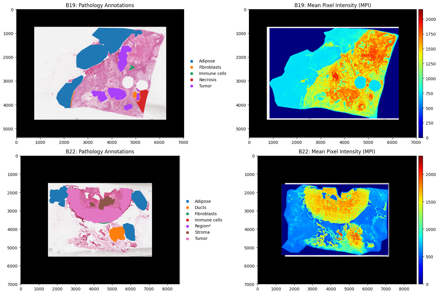
Now our data is loaded we can plot each dataset to visualise them
[4]:
fig, axes = plt.subplots(2, 2, figsize=(15, 10))

b19.pl.render_images("he_image")\
       .pl.render_shapes("annotations", color="classification")\
       .pl.show(ax=axes[0,0], title="B19: Pathology Annotations")

b22.pl.render_images("he_image")\
       .pl.render_shapes("annotations", color="classification")\
       .pl.show(ax=axes[1,0], title="B22: Pathology Annotations")

b19.pl.render_images("he_image")\
       .pl.render_shapes("pixels",color="MPI", cmap = "jet")\
       .pl.show(ax=axes[0,1], title="B19: Mean Pixel Intensity (MPI)")

b22.pl.render_images("he_image")\
       .pl.render_shapes("pixels", color="MPI", cmap = "jet")\
       .pl.show(ax=axes[1,1], title="B22: Mean Pixel Intensity (MPI)")


plt.tight_layout()
plt.show()
INFO     Rasterizing image for faster rendering.
INFO     Rasterizing image for faster rendering.
INFO     Rasterizing image for faster rendering.
INFO     Using 'datashader' backend with 'None' as reduction method to speed up plotting. Depending on the
         reduction method, the value range of the plot might change. Set method to 'matplotlib' to disable this
         behaviour.
INFO     Using the datashader reduction "mean". "max" will give an output very close to the matplotlib result.
Data Preprocessing#
Based on the plots above we can see that there is some noise (pixels with intensity readings) outside the tissue. The first step is to remove these pixels. The most common approach is to use PCA or clustering to identify a group of pixels outside the tissue and then filter out this cluster. Lets run goatpy spatial clustering:
[5]:
b19 = gp.graphpca_spatialdata(b19, tables= "maldi_adata",
    library_id= 'spatial',
    n_components = 50,
    n_neighbors = 8,
    alpha = 0.5)
b19 = gp.get_kmean_clusters(b19, tables= "maldi_adata",n_clusters = 8)

b22 = gp.graphpca_spatialdata(b22, tables= "maldi_adata",
    library_id= 'spatial',
    n_components = 50,
    n_neighbors = 8,
    alpha = 0.5)
b22 = gp.get_kmean_clusters(b22, tables= "maldi_adata",n_clusters = 8)
[6]:
fig, axs = plt.subplots(1, 2, figsize=(12, 6))

sc.pl.spatial(b19.tables["maldi_adata"], img_key="hires",
              color=["GPCA_clusters"], size=2, spot_size=5,
              alpha_img=0, ax=axs[0], show=False)


sc.pl.spatial(b22.tables["maldi_adata"], img_key="hires",
              color=["GPCA_clusters"], size=2, spot_size=5,
              alpha_img=0, ax=axs[1], show=False)
/var/folders/f1/3f7gj1393nb0phh8vzn910nm0000gn/T/ipykernel_87137/2307341997.py:3: FutureWarning: Use `squidpy.pl.spatial_scatter` instead.
  sc.pl.spatial(b19.tables["maldi_adata"], img_key="hires",
/var/folders/f1/3f7gj1393nb0phh8vzn910nm0000gn/T/ipykernel_87137/2307341997.py:8: FutureWarning: Use `squidpy.pl.spatial_scatter` instead.
  sc.pl.spatial(b22.tables["maldi_adata"], img_key="hires",
[6]:
[<Axes: title={'center': 'GPCA_clusters'}, xlabel='spatial1', ylabel='spatial2'>]
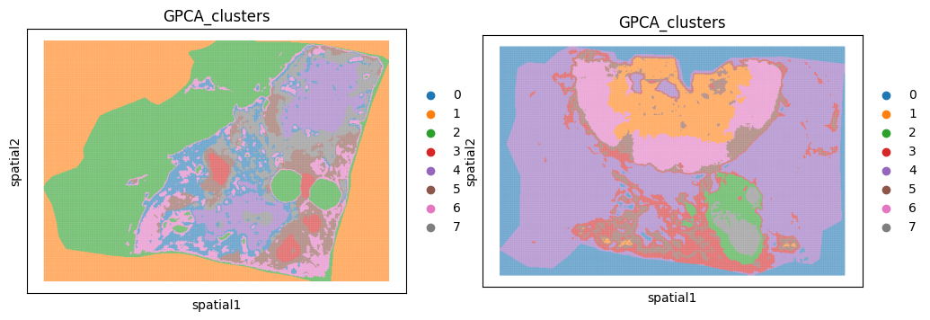
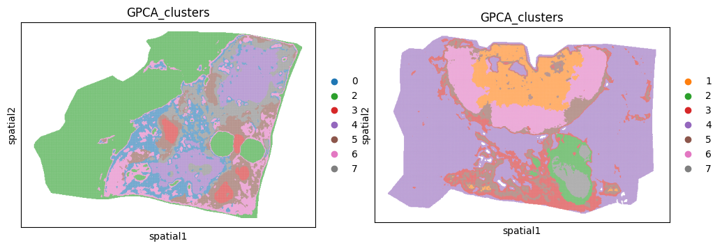
We can see that cluster 1 and 0 are outside the tissue section for sample b19 and b22 respecitively. We can use the function gp.filter_spatialdata implemented in goatpy to remove these clusters for each sample:
[7]:
b19 = gp.filter_spatialdata(b19, "GPCA_clusters != '1'")
b22 = gp.filter_spatialdata(b22, "GPCA_clusters != '0'")
  137,917 / 204,876 pixels selected (67.3%)
  Done. Result: SpatialData object

├── Images
│     └── 'he_image': DataArray[cyx] (3, 5380, 7020)
├── Points
│     └── 'centroids': DataFrame with shape: (<Delayed>, 3) (2D points)
├── Shapes
│     ├── 'annotations': GeoDataFrame shape: (24, 3) (2D shapes)
│     └── 'pixels': GeoDataFrame shape: (137917, 2) (2D shapes)
└── Tables
      └── 'maldi_adata': AnnData (137917, 128)
with coordinate systems:
    ▸ 'global', with elements:
        he_image (Images), centroids (Points), annotations (Shapes), pixels (Shapes)


  186,146 / 224,652 pixels selected (82.9%)
  Done. Result: SpatialData object

├── Images
│     └── 'he_image': DataArray[cyx] (3, 7000, 8670)
├── Points
│     └── 'centroids': DataFrame with shape: (<Delayed>, 3) (2D points)
├── Shapes
│     ├── 'annotations': GeoDataFrame shape: (17, 3) (2D shapes)
│     └── 'pixels': GeoDataFrame shape: (186146, 2) (2D shapes)
└── Tables
      └── 'maldi_adata': AnnData (186146, 123)
with coordinate systems:
    ▸ 'global', with elements:
        he_image (Images), centroids (Points), annotations (Shapes), pixels (Shapes)
Lets visualise the data with the background removed:
[8]:
fig, axs = plt.subplots(1, 2, figsize=(12, 6))

sc.pl.spatial(b19.tables["maldi_adata"], img_key="hires",
              color=["GPCA_clusters"], size=2, spot_size=5,
              alpha_img=0, ax=axs[0], show=False)


sc.pl.spatial(b22.tables["maldi_adata"], img_key="hires",
              color=["GPCA_clusters"], size=2, spot_size=5,
              alpha_img=0, ax=axs[1], show=False)
/var/folders/f1/3f7gj1393nb0phh8vzn910nm0000gn/T/ipykernel_87137/2307341997.py:3: FutureWarning: Use `squidpy.pl.spatial_scatter` instead.
  sc.pl.spatial(b19.tables["maldi_adata"], img_key="hires",
/var/folders/f1/3f7gj1393nb0phh8vzn910nm0000gn/T/ipykernel_87137/2307341997.py:8: FutureWarning: Use `squidpy.pl.spatial_scatter` instead.
  sc.pl.spatial(b22.tables["maldi_adata"], img_key="hires",
[8]:
[<Axes: title={'center': 'GPCA_clusters'}, xlabel='spatial1', ylabel='spatial2'>]
After filtering out pixels outside the tissue the next step is to nromalise the data. goatpy has gp.normalize_spatialdata, an inbuilt function for normalising data using either ‘TIC’ (total ion current) or ‘RMS’ (root mean squares) normalisation. Below is an example of how to use either method:
[9]:
sdata_tic = gp.normalize_spatialdata(
    b19,
    table_name="maldi_adata",
    method="TIC"
)

sdata_rms = gp.normalize_spatialdata(
    b19,
    table_name="maldi_adata",
    method="RMS"
)
[10]:
fig, axs = plt.subplots(1, 3, figsize=(15, 5))

sc.pl.spatial(b19.tables["maldi_adata"], img_key="hires",
              color="1136.559",  size=3,
              alpha_img=0, ax=axs[0], show=False, title = "Unnormalised Data")

sc.pl.spatial(sdata_tic.tables["maldi_adata"], img_key="hires",
              color="1136.559", size=3,
              alpha_img=0, ax=axs[1], show=False, title = "TIC Normalised Data")

sc.pl.spatial(sdata_rms.tables["maldi_adata"], img_key="hires",
              color="1136.559",  size=3,
              alpha_img=0, ax=axs[2], show=False, title = "RMS Normalised Data")
/var/folders/f1/3f7gj1393nb0phh8vzn910nm0000gn/T/ipykernel_75950/18049727.py:3: FutureWarning: Use `squidpy.pl.spatial_scatter` instead.
  sc.pl.spatial(b19.tables["maldi_adata"], img_key="hires",
/var/folders/f1/3f7gj1393nb0phh8vzn910nm0000gn/T/ipykernel_75950/18049727.py:7: FutureWarning: Use `squidpy.pl.spatial_scatter` instead.
  sc.pl.spatial(sdata_tic.tables["maldi_adata"], img_key="hires",
/var/folders/f1/3f7gj1393nb0phh8vzn910nm0000gn/T/ipykernel_75950/18049727.py:11: FutureWarning: Use `squidpy.pl.spatial_scatter` instead.
  sc.pl.spatial(sdata_rms.tables["maldi_adata"], img_key="hires",
[10]:
[<Axes: title={'center': 'RMS Normalised Data'}, xlabel='spatial1', ylabel='spatial2'>]
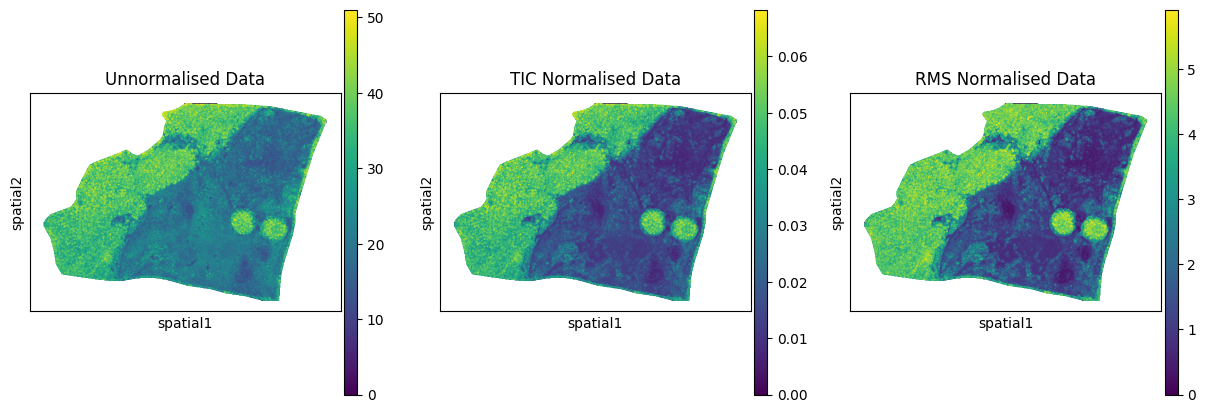
We can see above how either ‘TIC’ or ‘RMS’ normalisation effects the data. For this example we will use ‘TIC’ normalisation:
[11]:
b19_filtered = gp.normalize_spatialdata(b19, table_name="maldi_adata", method="TIC")
b22_filtered = gp.normalize_spatialdata(b22, table_name="maldi_adata", method="TIC")
Merging Data#
After preprocessing and normalisation of each dataset, we can merge them into one object to identify common clusterings/biological regions between each tissue.
Merging the dataset first is also importent to identify if there are any batch effects present between samples. If so, it is necessary to correct for these batch effects before performing any more downsteam analysis.
[12]:
merged = gp.merge_spatialdata(
    sdatas=[b19_filtered, b22_filtered],
    batch_names=["batch1", "batch2"]
    )
Feature summary:
  Common to all batches   : 92
  Total across all batches: 159
  Unique to batch1              : 36
  Unique to batch2              : 31
  feature_join='inner' → keeping common features only
  [batch1] alignment OK: 137,917 pixels, he_x[0]=3565.0, X[0,0]=0.0000
  [batch2] alignment OK: 186,146 pixels, he_x[0]=2475.0, X[0,0]=0.0000
  [batch1] post-concat alignment verified ✓
  [batch2] post-concat alignment verified ✓

Merged 2 SpatialData objects:
  batch1: 137,917 pixels
  batch2: 186,146 pixels
  Total pixels  : 324,063
  Total features: 92
  Images : ['he_image_batch1', 'he_image_batch2']
  Shapes : ['annotations_batch1', 'pixels_batch1', 'annotations_batch2', 'pixels_batch2']
  Points : ['centroids_batch1', 'centroids_batch2']
[13]:
merged
[13]:
SpatialData object
├── Images
│     ├── 'he_image_batch1': DataArray[cyx] (3, 5380, 7020)
│     └── 'he_image_batch2': DataArray[cyx] (3, 7000, 8670)
├── Points
│     ├── 'centroids_batch1': DataFrame with shape: (<Delayed>, 3) (2D points)
│     └── 'centroids_batch2': DataFrame with shape: (<Delayed>, 3) (2D points)
├── Shapes
│     ├── 'annotations_batch1': GeoDataFrame shape: (24, 3) (2D shapes)
│     ├── 'annotations_batch2': GeoDataFrame shape: (17, 3) (2D shapes)
│     ├── 'pixels_batch1': GeoDataFrame shape: (137917, 2) (2D shapes)
│     └── 'pixels_batch2': GeoDataFrame shape: (186146, 2) (2D shapes)
└── Tables
      └── 'maldi_adata': AnnData (324063, 92)
with coordinate systems:
    ▸ 'global', with elements:
        he_image_batch1 (Images), he_image_batch2 (Images), centroids_batch1 (Points), centroids_batch2 (Points), annotations_batch1 (Shapes), annotations_batch2 (Shapes), pixels_batch1 (Shapes), pixels_batch2 (Shapes)
We can see that our datset has been merged, whereby data from each layer has been combined in the one SpatialData object. Each element has also been uniquely defined based on the batch_names provided.
Now we have our merged object we can check if there are any obvious batch effects present:
[14]:
gp.check_batch(merged)
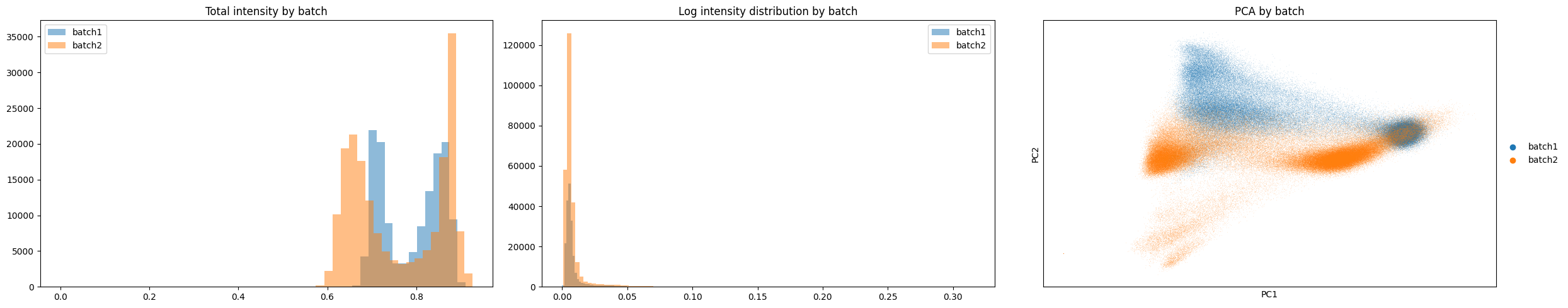
The above plots show a clear batch effect between our two samples as they do not share the same distributions across each plot, in particular the PCA plot.
To fully check if batch effects are present we can perform clustering with the merged dataset.
Using scanpy function with goatpy#
scanpy is a very popular spatial-omics analysis tool built using python. scanpy functions take Anndata objects, which for any goatpy object is stored in the Tables section under ‘maldi_adata’. This means any function in the scanpy universe or any other tool that inputs Anndata objects (i.e. squidpy, MALDIpy, stlearn, etc.) can be used with goatpy. For more infomation/tutorials on how to use Anndata objects with scanpy please visit
here.
Below we will run the common scanpy pipeline for clustering (originally designed for single-cell RNA data).
[15]:
## Run Clustering using scanpy pipeline
sc.pp.pca(merged["maldi_adata"])
sc.pp.neighbors(merged["maldi_adata"], n_neighbors=15)
sc.tl.umap(merged["maldi_adata"])
sc.tl.leiden(merged["maldi_adata"], resolution=0.2, key_added="leiden")
Now lets plot these results on UMAPs below:
[16]:
fig, axes = plt.subplots(1, 2, figsize=(14, 5))
sc.pl.umap(merged["maldi_adata"], color="leiden", ax=axes[0], show=False, title="Clusters")
sc.pl.umap(merged["maldi_adata"], color="batch", ax=axes[1], show=False, title="Batch")
plt.tight_layout()
plt.show()
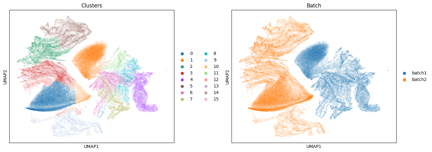
Based on these results and the plots above we can see there are clear batch effects between our samples with no clusters being shared between the two samples.
Due to this we should run some form of batch correction.
Batch Correction with goatpy#
There are various methods for performing batch correction on spatial-omics data. Two of the main methods which have displayed success when handleing MALDI-MSI data are ‘harmony’ and ‘ComBat’. These are two very different methods of batch correction. Breifly,
Harmony:
Iteratively moves cells/pixels in PCA space to mix batches while preserving local biological structure.
Harmony adjusts embeddings
Best used for clustering between samples
Combat:
Uses an empirical Bayes linear model to estimate and remove batch effects individually per feature.
Combat adjusts feature matrix
Best used for adjusting scaling differences in intensity values for differential abundance analysis.
Each method has its pros and cons, and should be selected with careful consideration based on the samples at hand. goatpy implements either method in the gp.batch_correction function.
Bellow we will run Harmony as an example:
[17]:
batch_corrected = gp.batch_correction(
    sdatas=[b19_filtered, b22_filtered],
    batch_names=["batch1", "batch2"],
    method="harmony", # or "combat"
    feature_join = "inner",
    pcs=30,
)
/var/folders/f1/3f7gj1393nb0phh8vzn910nm0000gn/T/ipykernel_12214/2099649585.py:1: UserWarning:
batch_correction assumes the data has already been normalised.
Running on raw counts may produce misleading results.
  batch_corrected = gp.batch_correction(
[0.23GB] Merging 2 SpatialData objects
Feature summary:
  Common to all batches   : 92
  Total across all batches: 159
  Unique to batch1              : 36
  Unique to batch2              : 31
  feature_join='inner' → keeping common features only
  [batch1] alignment OK: 137,917 pixels, he_x[0]=3565.0, X[0,0]=0.0000
  [batch2] alignment OK: 186,146 pixels, he_x[0]=2475.0, X[0,0]=0.0000
  [batch1] post-concat alignment verified ✓
  [batch2] post-concat alignment verified ✓

Merged 2 SpatialData objects:
  batch1: 137,917 pixels
  batch2: 186,146 pixels
  Total pixels  : 324,063
  Total features: 92
  Images : ['he_image_batch1', 'he_image_batch2']
  Shapes : ['annotations_batch1', 'pixels_batch1', 'annotations_batch2', 'pixels_batch2']
  Points : ['centroids_batch1', 'centroids_batch2']

[2.31GB] Input matrix: 324,063 pixels × 92 features
[2.31GB] Detected 2 batches
[2.32GB] Harmony input: 324,063 pixels × 92 features
[2.47GB] Detected 2 batches
[2.39GB] Scaled batch 'batch1' (137,917 pixels)
[2.40GB] Scaled batch 'batch2' (186,146 pixels)
[2.43GB] Running PCA (30 PCs)
2026-05-29 11:11:16,687 - harmonypy - INFO - Running Harmony (PyTorch on mps)
2026-05-29 11:11:16,688 - harmonypy - INFO -   Parameters:
2026-05-29 11:11:16,688 - harmonypy - INFO -     max_iter_harmony: 20
2026-05-29 11:11:16,688 - harmonypy - INFO -     max_iter_kmeans: 20
2026-05-29 11:11:16,689 - harmonypy - INFO -     epsilon_cluster: 1e-05
2026-05-29 11:11:16,689 - harmonypy - INFO -     epsilon_harmony: 0.0001
2026-05-29 11:11:16,689 - harmonypy - INFO -     nclust: 100
2026-05-29 11:11:16,690 - harmonypy - INFO -     block_size: 0.05
2026-05-29 11:11:16,690 - harmonypy - INFO -     lamb: [1. 1.]
2026-05-29 11:11:16,691 - harmonypy - INFO -     theta: [2. 2.]
2026-05-29 11:11:16,692 - harmonypy - INFO -     sigma: [0.1 0.1 0.1 0.1 0.1]...
2026-05-29 11:11:16,692 - harmonypy - INFO -     verbose: True
2026-05-29 11:11:16,692 - harmonypy - INFO -     random_state: 0
2026-05-29 11:11:16,692 - harmonypy - INFO -   Data: 30 PCs × 324063 cells
2026-05-29 11:11:16,693 - harmonypy - INFO -   Batch variables: ['batch']
[2.52GB] Running Harmony
2026-05-29 11:11:17,550 - harmonypy - INFO - Computing initial centroids with sklearn.KMeans...
2026-05-29 11:11:20,505 - harmonypy - INFO - KMeans initialization complete.
2026-05-29 11:11:20,723 - harmonypy - INFO - Iteration 1 of 20
2026-05-29 11:11:24,882 - harmonypy - INFO - Iteration 2 of 20
2026-05-29 11:11:28,966 - harmonypy - INFO - Iteration 3 of 20
2026-05-29 11:11:33,276 - harmonypy - INFO - Iteration 4 of 20
2026-05-29 11:11:37,212 - harmonypy - INFO - Iteration 5 of 20
2026-05-29 11:11:41,089 - harmonypy - INFO - Iteration 6 of 20
2026-05-29 11:11:45,143 - harmonypy - INFO - Iteration 7 of 20
2026-05-29 11:11:49,241 - harmonypy - INFO - Iteration 8 of 20
2026-05-29 11:11:52,024 - harmonypy - INFO - Converged after 8 iterations
[0.39GB] Harmony complete (embedding shape=(324063, 30))
[0.42GB] batch_correction complete (method='harmony')
After Harmony has been run on our samples we can check if these batch effects have been resolved in our corrected object.
Lets run gp.check_batch on our merged and batch corrected samples, and compare the differences:
[18]:
print("Non-Corrected Merged Data")
gp.check_batch(merged)

print("Batch-Corrected Data")
gp.check_batch(batch_corrected)
Non-Corrected Merged Data

Batch-Corrected Data
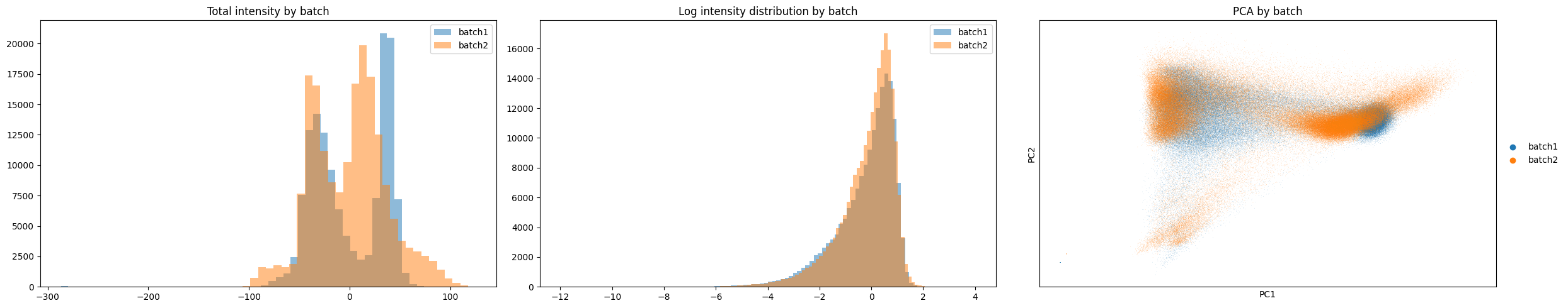
Based on the plots above we can see there is a clear improvement between the distributions of the two samples. Lets run clustering below and check if we see improved clustering across samples
[19]:
batch_corrected["maldi_adata"]
[19]:
AnnData object with n_obs × n_vars = 324063 × 159
    obs: 'x', 'y', 'MPI', 'he_x', 'he_y', 'instance_id', 'region', 'GPCA_clusters', 'batch'
    uns: 'pca', 'batch_correction'
    obsm: 'GraphPCA', 'spatial', 'X_pca', 'X_pca_harmony'
    varm: 'PCs'
After printing the ‘batch_corrected’ Anndata object stored in Tables, the corrected PCA embeddings required for clustering are stored under ‘X_pca_harmony’. We will need these for running the scanpy clustering pipeline below:
[20]:
sc.pp.neighbors(batch_corrected["maldi_adata"], use_rep="X_pca_harmony", n_neighbors=15)
sc.tl.umap(batch_corrected["maldi_adata"])
sc.tl.leiden(batch_corrected["maldi_adata"], resolution=0.3, key_added="leiden_harmony")

# Plot UMAP
fig, axes = plt.subplots(1, 2, figsize=(14, 5))
sc.pl.umap(batch_corrected["maldi_adata"], color="leiden_harmony", ax=axes[0], show=False, title="Clusters")
sc.pl.umap(batch_corrected["maldi_adata"], color="batch", ax=axes[1], show=False, title="Batch")
plt.tight_layout()
plt.show()
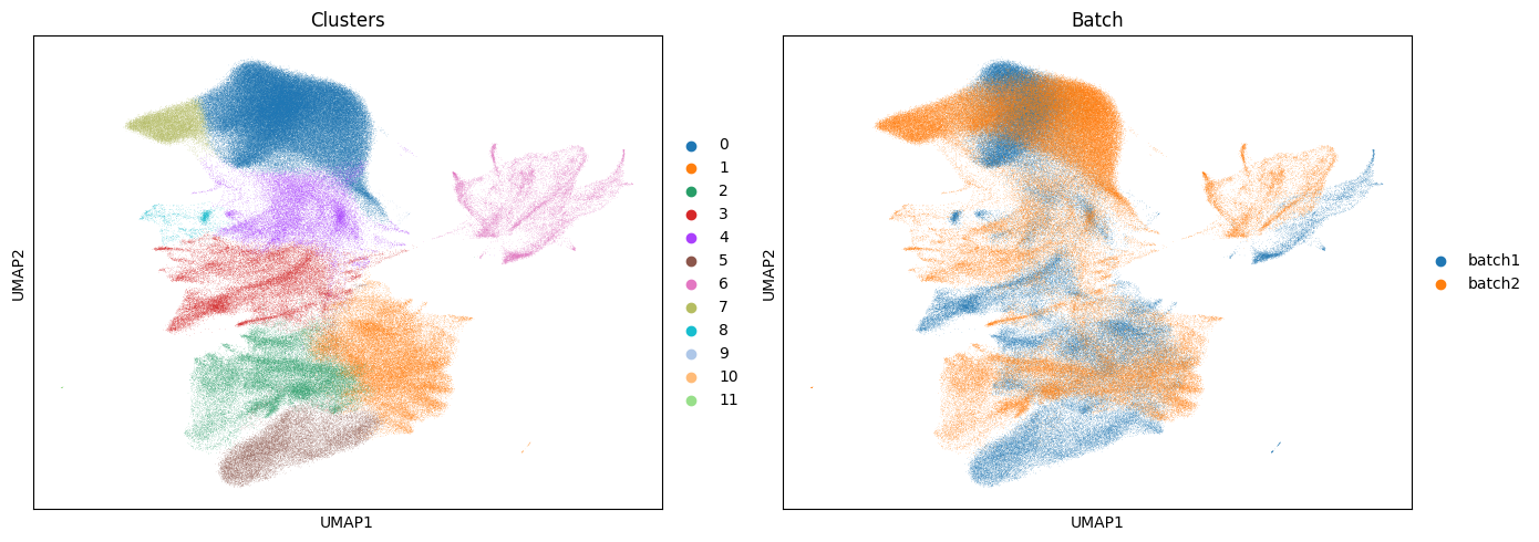
Based on the UMAP plots above we can see the batch effect has been removed between the samples, whereby we now have cluster that are shared between each sample.
[21]:
import pandas as pd
import matplotlib.pyplot as plt

# Get counts
counts = (
    batch_corrected["maldi_adata"].obs
    .groupby(["leiden_harmony", "batch"])
    .size()
    .unstack(fill_value=0)
)

# Plot stacked barplot
ax = counts.plot(kind="bar",stacked=True,figsize=(7, 3))

ax.set_xlabel("Leiden cluster")
ax.set_ylabel("Number of pixels")
ax.set_title("Batch composition per Harmony cluster")

plt.tight_layout()
plt.show()
/var/folders/f1/3f7gj1393nb0phh8vzn910nm0000gn/T/ipykernel_12214/1094874097.py:7: FutureWarning: The default of observed=False is deprecated and will be changed to True in a future version of pandas. Pass observed=False to retain current behavior or observed=True to adopt the future default and silence this warning.
  .groupby(["leiden_harmony", "batch"])
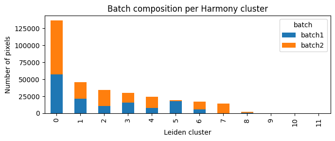
Lets visualise the new clusters spatially
[22]:
# Per-object spatial plots (if you have spatial coords)
sc.pl.spatial(batch_corrected["maldi_adata"], color="leiden_harmony",spot_size = 15, title="Harmony Clusters")
/var/folders/f1/3f7gj1393nb0phh8vzn910nm0000gn/T/ipykernel_12214/870433464.py:2: FutureWarning: Use `squidpy.pl.spatial_scatter` instead.
  sc.pl.spatial(batch_corrected["maldi_adata"], color="leiden_harmony",spot_size = 15, title="Harmony Clusters")
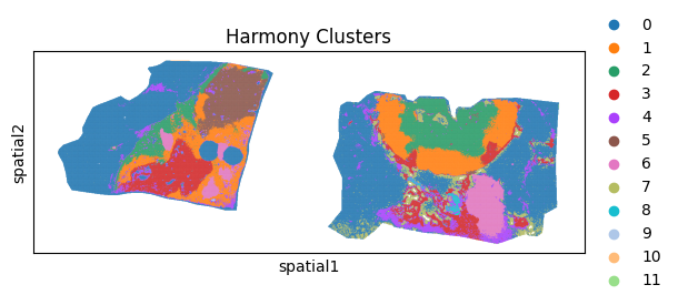
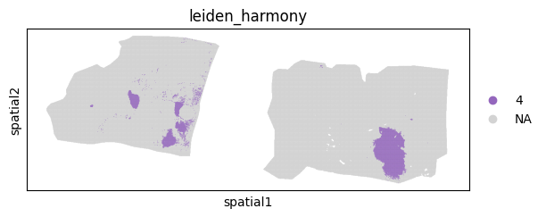
Using the method below we can also plot specific individual clusters into the tissue. Lets try with cluster 4:
[23]:
sc.pl.spatial(batch_corrected["maldi_adata"],groups=["4"], spot_size = 15, color="leiden_harmony")
/var/folders/f1/3f7gj1393nb0phh8vzn910nm0000gn/T/ipykernel_44848/1363687036.py:1: FutureWarning: Use `squidpy.pl.spatial_scatter` instead.
  sc.pl.spatial(batch_corrected["maldi_adata"],groups=["4"], spot_size = 15, color="leiden_harmony")
m/z peak glycan annotation#
Using goatpy’s curated glycan database we can annoate certain m/z values with a common glycan name. This can help improve batch correction and can be used for downstream analysis.
This dataset contains 173 glycans ranging from m/z of 933.32 to 3416.24. Alternatively, users can use their own glycan library to annotate certain m/z values.
Lets run the annotation function below:
[24]:
print(b19_filtered["maldi_adata"].var_names)
Index(['933.481', '1079.435', '1095.557', '1136.559', '1239.601', '1257.634',
       '1278.478', '1282.824', '1298.582', '1339.638',
       ...
       '3198.548', '3209.582', '3270.495', '3283.5', '3295.52', '3307.541',
       '3356.591', '3417.661', '3428.18', '3453.67'],
      dtype='object', length=128)
[25]:
b19_filtered = gp.annotate_glycans(b19_filtered)
b22_filtered = gp.annotate_glycans(b22_filtered)
Annotation Statistics
----------------------------------------
total_peaks: 128
annotated_peaks: 76
unannotated_peaks: 52
multi_annotation_peaks: 1
unique_glycans: 76
duplicate_glycans: 1
annotation_rate: 59.38

Duplicate Glycans
----------------------------------------
H4N5F1: 1828.819, 1850.877


Annotation Statistics
----------------------------------------
total_peaks: 123
annotated_peaks: 68
unannotated_peaks: 55
multi_annotation_peaks: 1
unique_glycans: 68
duplicate_glycans: 1
annotation_rate: 55.28

Duplicate Glycans
----------------------------------------
H4N5F1: 1828.819, 1850.877
Statistics are provided when running the gp.annotate_glycans function which state how many peaks got successfully annotated.
lets see how the feature names have be adjusted:
[26]:
print(b19_filtered["maldi_adata"].var_names)
Index(['H10N2', 'H3N2 (Man3)', 'H3N2F1 (Man3Fuc1)', 'H3N3', 'H3N3F1', 'H3N4',
       'H3N4F1', 'H3N5', 'H3N5F1', 'H3N6F1',
       ...
       'mz-3087.756', 'mz-3137.639', 'mz-3148.669', 'mz-3198.548', 'mz-3283.5',
       'mz-3295.52', 'mz-3307.541', 'mz-3417.661', 'mz-3428.18', 'mz-3453.67'],
      dtype='object', length=127)
Differential Abundance Analysis#
To run this analysis we will first annotate our harmony corrected dataset. This will help increase the number of common glycans shared between our two samples.
[27]:
batch_corrected = gp.annotate_glycans(batch_corrected)
Annotation Statistics
----------------------------------------
total_peaks: 92
annotated_peaks: 63
unannotated_peaks: 29
multi_annotation_peaks: 1
unique_glycans: 63
duplicate_glycans: 1
annotation_rate: 68.48

Duplicate Glycans
----------------------------------------
H4N5F1: 1828.819, 1850.877
We can see that 63 peaks were annotated correctly. Using this object plus the harmony corrected clusters as a covariate we can run ComBat to correct for varriation between glycan intensity distributions across samples.
[28]:
combat_corrected = gp.batch_correction(
    pre_merged=batch_corrected,
    batch_names=["batch1", "batch2"],
    method="combat",
    feature_join="inner",
    covariates= ["leiden_harmony"]
)
/var/folders/f1/3f7gj1393nb0phh8vzn910nm0000gn/T/ipykernel_54952/2093005718.py:1: UserWarning:
batch_correction assumes the data has already been normalised.
Running on raw counts may produce misleading results.
  combat_corrected = gp.batch_correction(
[0.97GB] Using pre-merged SpatialData object
[0.97GB] Input matrix: 324,063 pixels × 91 features
[0.93GB] Detected 2 batches
[0.73GB] Preserving covariates: ['leiden_harmony']
[0.73GB] Running ComBat (matrix shape=(324063, 91))
[0.87GB] Clipping 23,106 negative values to 0
[0.65GB] ComBat complete
[0.65GB] batch_correction complete (method='combat')
Now lets run differential abundance analysis:
[29]:
# run DAA
sc.tl.rank_genes_groups(combat_corrected["maldi_adata"], groupby='leiden_harmony', method='wilcoxon')
[30]:
sc.pl.rank_genes_groups(combat_corrected["maldi_adata"], n_genes=25, sharey=False)
[31]:
de_results = sc.get.rank_genes_groups_df(combat_corrected["maldi_adata"], group=None)
[32]:
de_results
[32]:
| group | names | scores | logfoldchanges | pvals | pvals_adj | |
|---|---|---|---|---|---|---|
| 0 | 0 | mz-1401.624 | 246.027817 | 0.476703 | 0.000000e+00 | 0.000000e+00 |
| 1 | 0 | mz-1679.73 | 234.151108 | 0.414342 | 0.000000e+00 | 0.000000e+00 |
| 2 | 0 | H3N2 (Man3) | 228.863983 | 0.553977 | 0.000000e+00 | 0.000000e+00 |
| 3 | 0 | mz-1629.766 | 228.429565 | 0.411559 | 0.000000e+00 | 0.000000e+00 |
| 4 | 0 | mz-1546.688 | 223.605209 | 0.387996 | 0.000000e+00 | 0.000000e+00 |
| ... | ... | ... | ... | ... | ... | ... |
| 996 | 10 | H3N5F1 | -8.436407 | -1.126163 | 3.272415e-17 | 4.582033e-16 |
| 997 | 10 | H5N4S2F1, H5N4Am1D1F1 | -8.442063 | -1.370445 | 3.117850e-17 | 4.582033e-16 |
| 998 | 10 | H4N3 | -8.444786 | -1.245456 | 3.046021e-17 | 4.582033e-16 |
| 999 | 10 | H5N5M1F1 | -8.467253 | -1.203054 | 2.512479e-17 | 4.582033e-16 |
| 1000 | 10 | H4N5F1 | -8.476522 | -1.091752 | 2.320249e-17 | 4.582033e-16 |
1001 rows × 6 columns
[33]:
import numpy as np
import matplotlib.pyplot as plt
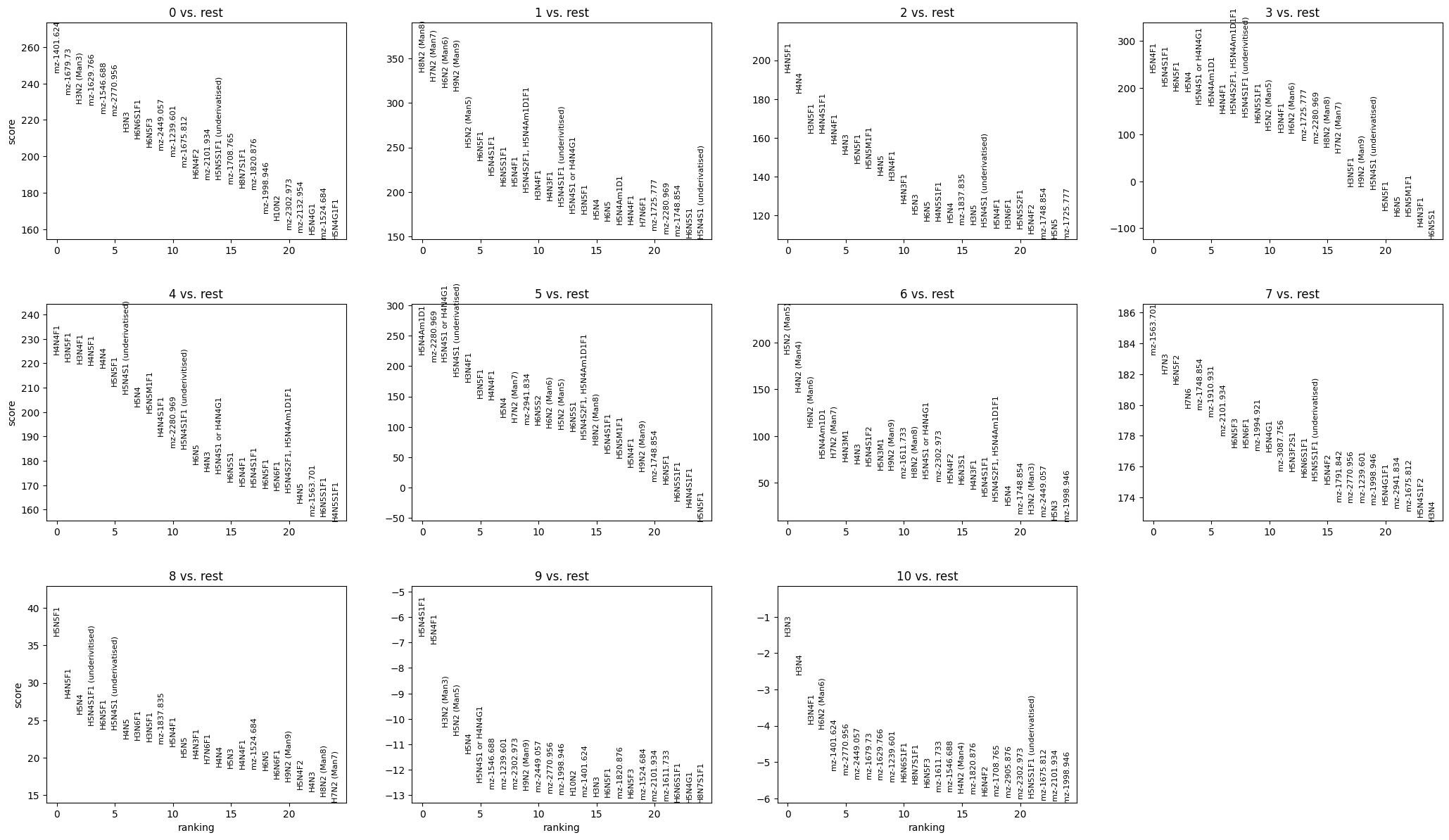
n_top = 5
top_markers = (
de_results
.sort_values(["group", "scores"], ascending=[True, False])
.groupby("group")
.head(n_top)
.copy()
)
top_markers["minus_log10_p"] = -np.log10(
top_markers["pvals_adj"].clip(lower=1e-300)
)
plt.figure(figsize=(10, 15))
scatter = plt.scatter(
x=top_markers["group"],
y=top_markers["names"],
s=top_markers["minus_log10_p"],
c=top_markers["logfoldchanges"],
cmap="RdBu_r"
)
plt.colorbar(scatter, label="logFC")
plt.xlabel("Cluster")
plt.ylabel("Feature")
plt.tight_layout()
plt.show()
/var/folders/f1/3f7gj1393nb0phh8vzn910nm0000gn/T/ipykernel_54952/1402176575.py:9: FutureWarning: The default of observed=False is deprecated and will be changed to True in a future version of pandas. Pass observed=False to retain current behavior or observed=True to adopt the future default and silence this warning.
  .groupby("group")
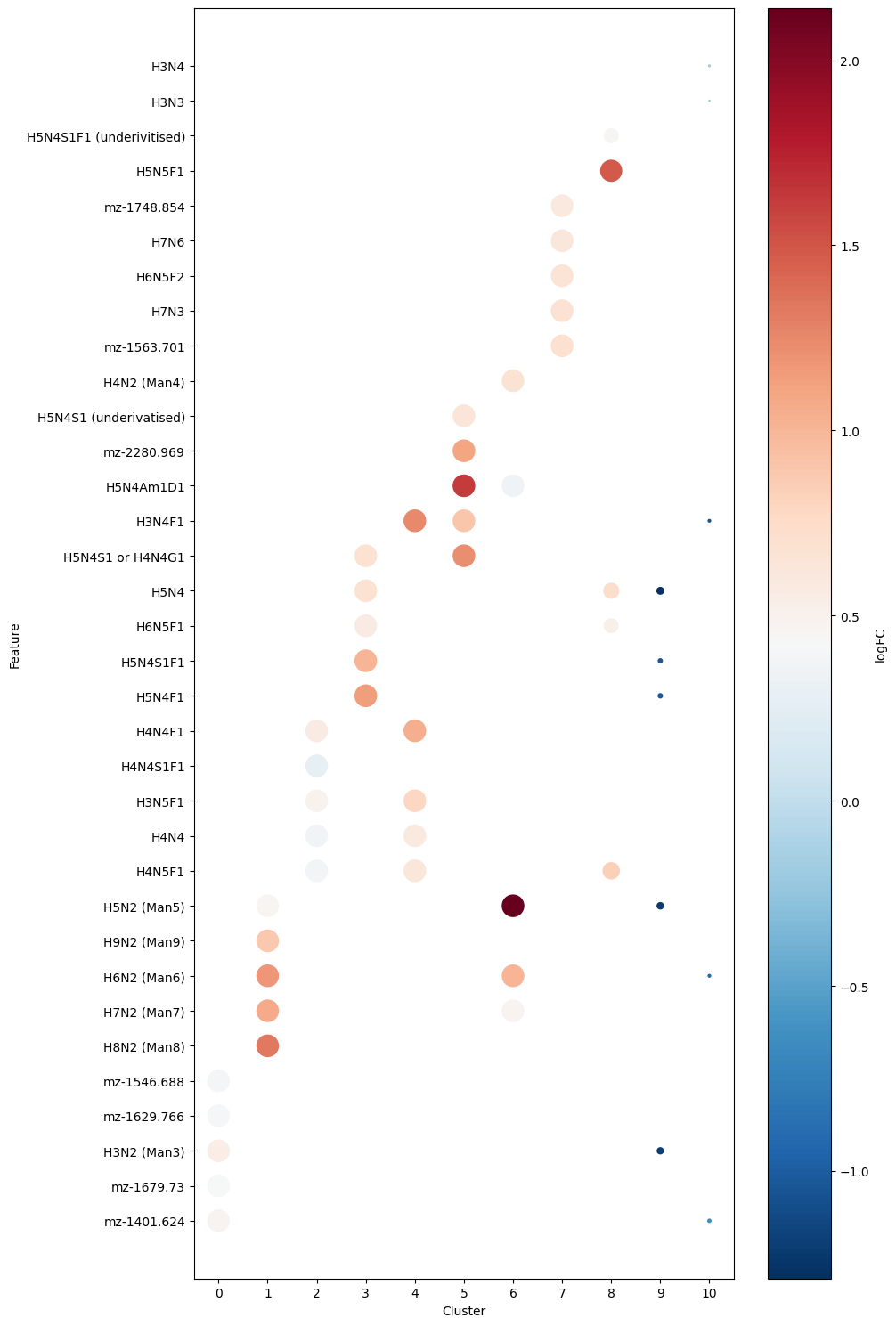
We can see the top 5 glycans for each cluster. Some were succesfully annotated whereas other are currently unknown. Regardless we can plot some of these key glycans spatially:
[34]:
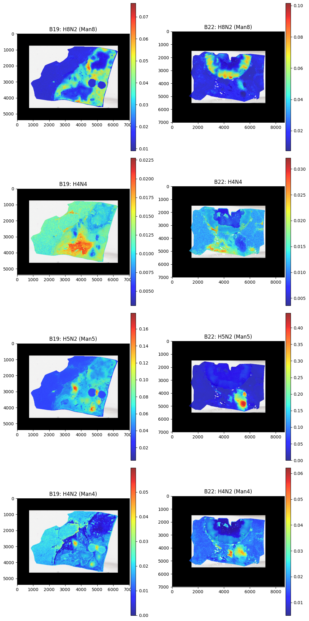
vals = ['H8N2 (Man8)','H4N4', 'H5N2 (Man5)','H4N2 (Man4)']

fig, axes = plt.subplots(4, 2, figsize=(10, 20))

for i,v in enumerate(vals):

    batch_corrected.pl.render_images("he_image_batch1")\
        .pl.render_shapes("pixels_batch1", color=v,cmap = "jet", fill_alpha = 0.8)\
        .pl.show(ax=axes[i,0], title=f"B19: {v}", )

    batch_corrected.pl.render_images("he_image_batch2")\
        .pl.render_shapes("pixels_batch2", color=v,cmap = "jet", fill_alpha = 0.8)\
        .pl.show(ax=axes[i,1], title=f"B22: {v}")


plt.tight_layout()
plt.show()
INFO     Rasterizing image for faster rendering.
INFO     Using 'datashader' backend with 'None' as reduction method to speed up plotting. Depending on the
         reduction method, the value range of the plot might change. Set method to 'matplotlib' to disable this
         behaviour.
INFO     Using the datashader reduction "mean". "max" will give an output very close to the matplotlib result.
Comparing Pathologist Annotation#
In addition to clusters we can also look into pathologist annotations, and determine differenitally abundant glycans in these regions.
To do this we must first run gp.annotations_to_pixels, to identify which annotations correspond to which pixel:
Note: This is best to run on individual objects and should be run prior to merging/batch correction
[ ]:
#b19_filtered = gp.annotations_to_pixels(b19_filtered)
#b22_filtered = gp.annotations_to_pixels(b22_filtered)
We can see in the example above after running we get a breakdown of the number and percentage of pixels that were annotated for each group. Lets see how they are stored in our merged object:
[36]:
batch_corrected['maldi_adata'].obs["annotation"]
[36]:
batch1_0         Adipose
batch1_1         Adipose
batch1_2         Adipose
batch1_3         Adipose
batch1_4         Adipose
                  ...
batch2_186141      other
batch2_186142      other
batch2_186143      other
batch2_186144      other
batch2_186145      other
Name: annotation, Length: 324063, dtype: category
Categories (9, object): ['Adipose', 'Ducts', 'Fibroblasts', 'Immune cells', ..., 'Region*', 'Stroma', 'Tumor', 'other']
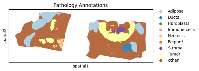
Stored in the annotation column, lets also visualise these results:
[37]:
sc.pl.spatial(batch_corrected["maldi_adata"], color="annotation",spot_size = 15, title="Pathology Annotations", palette="Paired")
/var/folders/f1/3f7gj1393nb0phh8vzn910nm0000gn/T/ipykernel_54952/2347659777.py:1: FutureWarning: Use `squidpy.pl.spatial_scatter` instead.
  sc.pl.spatial(batch_corrected["maldi_adata"], color="annotation",spot_size = 15, title="Pathology Annotations", palette="Paired")
Now that we have our annotated regions similar to before we can run differential abundance analysis:
[38]:
adata = batch_corrected["maldi_adata"].copy()

counts = adata.obs["annotation"].value_counts()
valid_groups = counts[counts > 1].index

adata = adata[adata.obs["annotation"].isin(valid_groups)].copy()

sc.tl.rank_genes_groups(
    adata,
    groupby="annotation",
    method="wilcoxon"
)

groups = adata.uns["rank_genes_groups"]["names"].dtype.names

top_features = []

for group in groups:
    genes = sc.get.rank_genes_groups_df(
        adata,
        group=group
    )["names"].head(5).tolist()

    top_features.extend(genes)

# Remove duplicates while preserving order
top_features = list(dict.fromkeys(top_features))
[39]:
sc.pl.heatmap(
    adata,
    var_names=top_features,
    groupby="annotation",
    standard_scale="var",
    cmap="RdBu_r",
    swap_axes=True,
    use_raw = False,
    log = True,
)
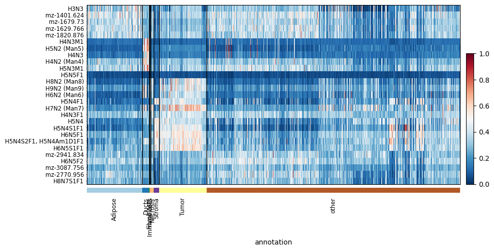
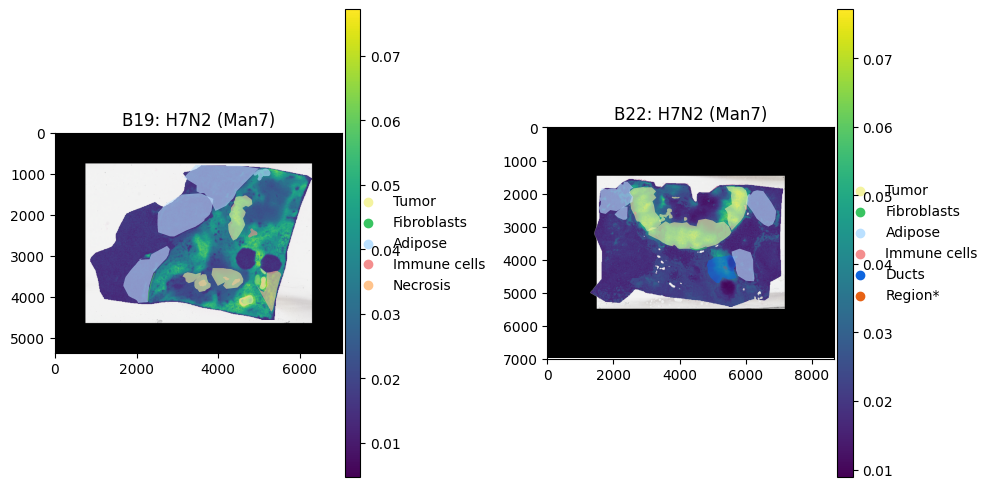
We can again see some key glycans that are highly express by the Tumour regions.
Another interesting fact shows that there may have been some tumour regions missed in the annotation process as there are some pixels in the ‘other’ region that have similar intenisty profiles.
Lets plot a key Tumour Glycan:
[40]:
palette = {
    "Tumor": "#f4f39f",   # red
    "Fibroblasts": "#39c461",   # green
    "Adipose": "#bae0ff",   # blue
    "Immune cells": "#f48e8e",  # purple
    "Necrosis": "#ffc38b",
    "Ducts": "#0e65de",
    "Region*": "#e76215",
    "other": "#773813",
}

groups = list(palette.keys())
colors = list(palette.values())


fig, axes = plt.subplots(1, 2, figsize=(10, 5))

batch_corrected.pl.render_images("he_image_batch1")\
        .pl.render_shapes("pixels_batch1", color='H7N2 (Man7)',cmap = "viridis", fill_alpha = 1)\
        .pl.render_shapes("annotations_batch1", color='classification',groups=groups,palette=colors, fill_alpha = 0.6)\
        .pl.show(ax=axes[0], title="B19: H7N2 (Man7)", )

batch_corrected.pl.render_images("he_image_batch2")\
        .pl.render_shapes("pixels_batch2", color='H7N2 (Man7)',cmap = "viridis", fill_alpha = 1)\
        .pl.render_shapes("annotations_batch2", color='classification',groups=groups,palette=colors, fill_alpha = 0.6)\
        .pl.show(ax=axes[1], title="B22: H7N2 (Man7)")

plt.tight_layout()
plt.show()
INFO     Rasterizing image for faster rendering.
INFO     Using 'datashader' backend with 'None' as reduction method to speed up plotting. Depending on the
         reduction method, the value range of the plot might change. Set method to 'matplotlib' to disable this
         behaviour.
INFO     Using the datashader reduction "mean". "max" will give an output very close to the matplotlib result.
INFO     Rasterizing image for faster rendering.
INFO     Using 'datashader' backend with 'None' as reduction method to speed up plotting. Depending on the
         reduction method, the value range of the plot might change. Set method to 'matplotlib' to disable this
         behaviour.
INFO     Using the datashader reduction "mean". "max" will give an output very close to the matplotlib result.
Tutorial Session Info#
[41]:
from session_info import show
show()
[41]:
Click to view session information
-----
goatpy              0.1.0
matplotlib          3.10.8
napari              0.6.6
napari_spatialdata  0.6.0
numpy               2.2.6
pandas              2.3.3
scanpy              1.11.5
session_info        v1.0.1
spatialdata         0.5.0
spatialdata_plot    0.2.12
squidpy             1.6.5
-----
Click to view modules imported as dependencies
81d243bd2c585b0f4821__mypyc NA
PIL                         12.1.1
PyQt5                       NA
ac51d50a4f4b6d748b8c__mypyc NA
anndata                     0.11.4
annotated_types             0.7.0
app_model                   0.4.0
appdirs                     1.4.4
appnope                     0.1.4
asciitree                   NA
asttokens                   NA
attr                        25.4.0
attrs                       25.4.0
babel                       2.18.0
backports                   NA
bermuda                     NA
cachey                      0.2.1
certifi                     2026.02.25
charset_normalizer          3.4.5
click                       8.3.1
cloudpickle                 3.1.2
colorama                    0.4.6
comm                        0.2.3
cv2                         4.13.0
cycler                      0.12.1
cython_runtime              NA
dask                        2024.11.2
dask_image                  NA
datashader                  0.18.2
dateutil                    2.9.0.post0
debugpy                     1.8.20
decorator                   5.2.1
distributed                 2024.11.2
docrep                      0.3.2
docstring_parser            NA
exceptiongroup              1.3.1
executing                   2.2.1
flexcache                   0.3
flexparser                  0.4
fsspec                      2026.2.0
geopandas                   1.1.2
h5py                        3.16.0
heapdict                    NA
hsluv                       5.0.4
idna                        3.11
igraph                      1.0.0
imagecodecs                 2025.3.30
imageio                     2.37.2
importlib_metadata          NA
in_n_out                    0.2.1
ipykernel                   6.31.0
jaraco                      NA
jedi                        0.19.2
jinja2                      3.1.6
joblib                      1.5.3
jsonschema                  4.26.0
jsonschema_specifications   NA
kiwisolver                  1.4.9
lazy_loader                 0.5
legacy_api_wrap             NA
leidenalg                   0.11.0
llvmlite                    0.46.0
locket                      NA
loguru                      0.7.3
lxml                        6.1.1
magicgui                    0.10.1
markupsafe                  3.0.3
matplotlib_scalebar         0.9.0
metaspace                   2.0.9
metaspace_converter         NA
more_itertools              10.8.0
mpl_toolkits                NA
msgpack                     1.1.2
multipledispatch            0.6.0
multiscale_spatial_image    2.0.3
napari_builtins             0.6.6
napari_plugin_engine        0.2.1
natsort                     8.4.0
networkx                    3.4.2
npe2                        0.8.1
numba                       0.64.0
numcodecs                   0.13.1
numpydoc                    1.10.0
ome_zarr                    NA
packaging                   26.0
parso                       0.8.6
patsy                       1.0.2
pims                        0.7
pint                        0.24.4
pkg_resources               NA
platformdirs                4.9.4
plotly                      6.6.0
prompt_toolkit              3.0.52
psutil                      7.2.2
psygnal                     0.15.1
pure_eval                   0.2.3
pyarrow                     21.0.0
pyct                        0.6.0
pydantic                    2.12.5
pydantic_compat             0.1.2
pydantic_core               2.41.5
pydantic_extra_types        2.11.0
pydev_ipython               NA
pydevconsole                NA
pydevd                      3.2.3
pydevd_file_utils           NA
pydevd_plugins              NA
pydevd_tracing              NA
pygments                    2.19.2
pyimzml                     1.5.5
pyparsing                   3.3.2
pyproj                      3.7.1
pyqtgraph                   0.14.0
pytz                        2026.1.post1
qtpy                        2.4.3
referencing                 NA
requests                    2.32.5
rich                        NA
rpds                        NA
scipy                       1.15.3
seaborn                     0.13.2
shapely                     2.1.2
sip                         NA
six                         1.17.0
skimage                     0.25.2
sklearn                     1.7.2
slicerator                  1.1.0
sopa                        2.1.11
sortedcontainers            2.4.0
spatial_image               1.2.3
sphinxcontrib               NA
stack_data                  0.6.3
statsmodels                 0.14.6
superqt                     0.8.0
tblib                       3.2.2
texttable                   1.7.0
threadpoolctl               3.6.0
tifffile                    2025.5.10
tlz                         1.1.0
toolz                       1.1.0
torch                       2.10.0
torchgen                    NA
tornado                     6.5.4
tqdm                        4.67.3
traitlets                   5.14.3
triangle                    20250106
typing_extensions           NA
typing_inspection           NA
urllib3                     2.6.3
validators                  0.35.0
vispy                       0.15.2
vscode                      NA
wcwidth                     0.6.0
wrapt                       2.1.2
xarray                      2025.6.1
xarray_dataclass            3.0.0
xarray_schema               0.0.3
xrspatial                   0.5.3
yaml                        6.0.3
zarr                        2.18.3
zict                        3.0.0
zipp                        NA
zmq                         27.1.0
zoneinfo                    NA
-----
IPython             8.38.0
jupyter_client      8.8.0
jupyter_core        5.9.1
-----
Python 3.10.19 | packaged by conda-forge | (main, Oct 22 2025, 22:46:49) [Clang 19.1.7 ]
macOS-26.3.1-arm64-arm-64bit
-----
Session information updated at 2026-06-04 14:02