Getting Started with goatpy Tutorial#
Author:Andrew Causer
This notebook is a tutorial of how to use goatpy for analysing Glycomics data and aligning the data with a H&E image. First make sure you have setup a conda evironement containing all the packages required for running GOATpy. For instructions on how to do this please visit the README.md file on agc888/goatpy.
Once this is done you can install the package with:
pip install goatpy
Data objects generated using goatpy build on the popular spaital-omics data package SpatialData and Anndata. Breifly, SpatialData is a package that efficently stores spatial datasets containing numerous layers of data. In particular, those with matching spatail expression/inensity data and image data. This data is stored in 4 main slots, those being Images, Shapes, Points and Tables. Examples of what each of these layers may store are:
Images- H&E or IHC imagesShapes- MALDI pixels, Pathologist annotations, in-tissue polygons, ROI regionsPoints- Pixel centroids, spatail data points, trajectory start/end pointsTables- Anndata object containing intensity values, additional pixel-based metadata (clustering, batch, MPI, etc.)
Tables is quite an important slot as it stores an Anndata object containing the expression/intensity values of Spatial Glycomics. Anndata is another key data stucture class as it is used by many popular downstream analysis python package including scanpy, squidpy, etc. For more infomation please visit some of the links below:
[1]:
import goatpy as gp
import spatialdata_plot
import matplotlib.pyplot as plt
import scanpy as sc
import pandas as pd
import squidpy as sq
from napari_spatialdata import Interactive
Loading and Aligning Data#
There are 2 main methods to load and align MALDI and a H&E image using goatpy. These are:
Automatic alignment (most simple approach) - this involves the loading and alignment of datasets without the need for manual point picking.
Manual alignent (more involved)- this involves loading the MALDI and H&E seperatlly and using
naparito perform manual landmark-basaed alignment
First we will demonstrate the automated loading and alignment approach.
Manual MALDI/H&E Alignment#
[2]:
path = "./Documents/AD_resolution_change_check_10um_actual_10012020_2.imzML"
he_path = "./Documents/res_check_0000.tif"

maldi_sd = gp.glyco_spatialdata(imzml_path=path)
he_sd = gp.he_spatialdata(he_path)
Successfully loaded with sopa.io.wsi
[3]:
maldi_sd
[3]:
SpatialData object
├── Points
│     └── 'centroids': DataFrame with shape: (<Delayed>, 112) (2D points)
├── Shapes
│     └── 'pixels': GeoDataFrame shape: (16455, 2) (2D shapes)
└── Tables
      └── 'maldi_adata': AnnData (16455, 108)
with coordinate systems:
    ▸ 'global', with elements:
        centroids (Points), pixels (Shapes)
[4]:
he_sd
[4]:
SpatialData object
└── Images
      └── 'he_image': DataTree[cyx] (3, 19160, 23633)
with coordinate systems:
    ▸ 'global', with elements:
        he_image (Images)
Above shows the structure of our two data object (MALDI and H&E). Lets visualise these below using SpatialData plotting.
[5]:
fig, axes = plt.subplots(1, 2, figsize=(10, 5))

he_sd.pl.render_images("he_image").pl.show(ax=axes[0], title="H&E Image")

maldi_sd.pl.render_shapes(color="MPI", cmap = "viridis")\
       .pl.show(ax=axes[1], title="MALDI Mean Pixel Intensity (MPI)")

plt.tight_layout()
plt.show()
INFO     Rasterizing image for faster rendering.
INFO     Using 'datashader' backend with 'None' as reduction method to speed up plotting. Depending on the
         reduction method, the value range of the plot might change. Set method to 'matplotlib' to disable this
         behaviour.
INFO     Using the datashader reduction "mean". "max" will give an output very close to the matplotlib result.
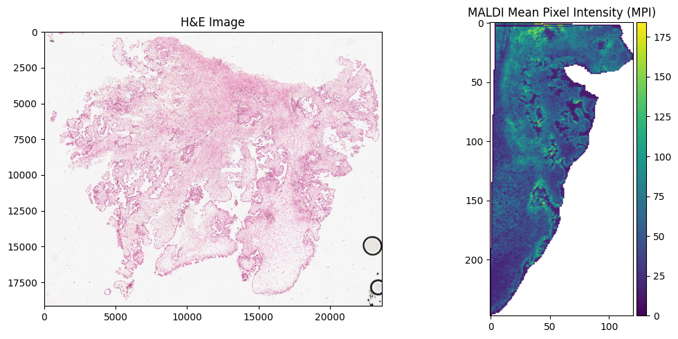
We can see above that the calls for currently plotting the data are pl.render_images and pl.render_shapes for the H&E image and MALDI pixels respecitively. Before aligning the MALDI data to the H&E image, we need to add a image layer to the MALDI SpatialData object, which comes in the form of a pseudo-image. This is because the landmark alignment function requires both SpatialData objects to have image layers. To generate a pseudo-image we can use two common datatypes, either MPI (mean
pixel intensity) or clustering results. TIC is automatically calculated when loading the data using glyco_spatialdata.
GOATpy has GraphPCA imbuilt which uses both spaital data and also glycan insnsity values to indifity similar clusters of pixels. Lets run that below
[6]:
maldi_sd = gp.graphpca_spatialdata(maldi_sd, tables= "maldi_adata",
    library_id= 'spatial',
    n_components = 50,
    n_neighbors = 15,
    alpha = 0.5)

maldi_sd = gp.get_kmean_clusters(maldi_sd, tables= "maldi_adata",n_clusters = 12)
After running the above lines our spatially informed clustering results will be stored in our Anndata object stored in the Tables section of our maldi_sd data object under the name ‘maldi_adata’. Specifically, the clustering results will be stored in the .obs section in a columnn called ‘GPCA_clusters’. Below shows the Anndata object structure and the .obs table respectively.
[7]:
maldi_sd["maldi_adata"]
[7]:
AnnData object with n_obs × n_vars = 16455 × 108
    obs: 'x', 'y', 'instance_id', 'region', 'full_x', 'full_y', 'MPI', 'GPCA_clusters'
    uns: 'spatialdata_attrs'
    obsm: 'spatial', 'GraphPCA'
[8]:
maldi_sd["maldi_adata"].obs
[8]:
| x | y | instance_id | region | full_x | full_y | MPI | GPCA_clusters | |
|---|---|---|---|---|---|---|---|---|
| 0 | 66 | 123 | 0 | pixels | 2705 | 1001 | 14.858001 | 10 |
| 1 | 67 | 123 | 1 | pixels | 2706 | 1001 | 16.228001 | 10 |
| 2 | 64 | 123 | 2 | pixels | 2703 | 1001 | 13.924000 | 3 |
| 3 | 65 | 123 | 3 | pixels | 2704 | 1001 | 12.410001 | 10 |
| 4 | 4 | 124 | 4 | pixels | 2643 | 1002 | 33.486004 | 1 |
| ... | ... | ... | ... | ... | ... | ... | ... | ... |
| 16450 | 51 | 56 | 16450 | pixels | 2690 | 934 | 16.430000 | 3 |
| 16451 | 56 | 56 | 16451 | pixels | 2695 | 934 | 84.561989 | 8 |
| 16452 | 57 | 56 | 16452 | pixels | 2696 | 934 | 38.590000 | 3 |
| 16453 | 54 | 56 | 16453 | pixels | 2693 | 934 | 60.991997 | 3 |
| 16454 | 55 | 56 | 16454 | pixels | 2694 | 934 | 51.322002 | 3 |
16455 rows × 8 columns
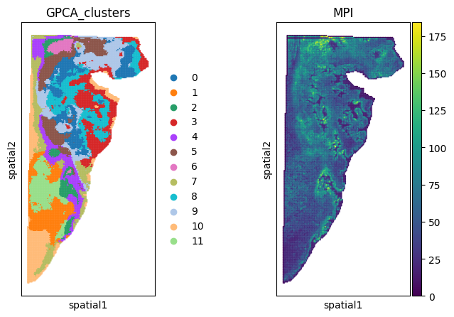
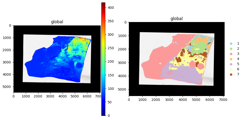
The clusters have been successfully stored in the ‘GPCA_clusters’ columnn. Lets use this to look at the results of the clustering and also our mean pixel intensity (MPI) values:
[9]:
fig, axs = plt.subplots(1, 2, figsize=(8, 5))

sc.pl.spatial(maldi_sd.tables["maldi_adata"], img_key="hires",
              color=["GPCA_clusters"], size=1.5, spot_size=1,
              alpha_img=0, ax=axs[0], show=False)


sc.pl.spatial(maldi_sd.tables["maldi_adata"], img_key="hires",
              color=["MPI"], size=1.5, spot_size=1,
              alpha_img=0, ax=axs[1], show=False)
/var/folders/f1/3f7gj1393nb0phh8vzn910nm0000gn/T/ipykernel_20678/2053279120.py:3: FutureWarning: Use `squidpy.pl.spatial_scatter` instead.
  sc.pl.spatial(maldi_sd.tables["maldi_adata"], img_key="hires",
/var/folders/f1/3f7gj1393nb0phh8vzn910nm0000gn/T/ipykernel_20678/2053279120.py:8: FutureWarning: Use `squidpy.pl.spatial_scatter` instead.
  sc.pl.spatial(maldi_sd.tables["maldi_adata"], img_key="hires",
[9]:
[<Axes: title={'center': 'MPI'}, xlabel='spatial1', ylabel='spatial2'>]
We need a pseudo-image from our maldi data to use to identify landmarks for image alignment, lets use the MPI results:
[10]:
maldi_sd = gp.Add_Pseudo_Image(maldi_sd, "MPI", tables = "maldi_adata", library_id = "Spatial", is_continous=True, cmap = "viridis",img_upscaling=50)
#maldi_sd = gp.Add_Pseudo_Image(maldi_sd, "GPCA_clusters", tables = "maldi_adata", library_id = "Spatial", cmap = "Paired")
INFO Transposing `data` of type: <class 'dask.array.core.Array'> to ('c', 'y', 'x').
[11]:
maldi_sd
[11]:
SpatialData object
├── Images
│     └── 'optical_image': DataTree[cyx] (3, 12400, 6000), (3, 6200, 3000), (3, 3100, 1500), (3, 1550, 750)
├── Points
│     └── 'centroids': DataFrame with shape: (<Delayed>, 112) (2D points)
├── Shapes
│     └── 'pixels': GeoDataFrame shape: (16455, 2) (2D shapes)
└── Tables
      └── 'maldi_adata': AnnData (16455, 108)
with coordinate systems:
    ▸ 'global', with elements:
        optical_image (Images), centroids (Points), pixels (Shapes)
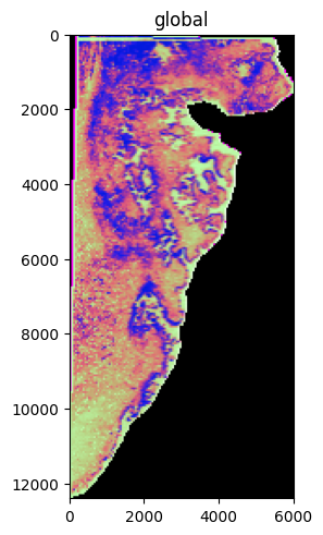
Our MALDI object now has a optical_image Image slot. Lets plot at the pseudo-image below:
[12]:
maldi_sd.pl.render_images("optical_image").pl.show()
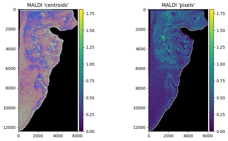
We can also plot a glycan value to visalise the image/pixel overlay. Here we plot centroid Points and pixels Shapes. The key difference is that with the Points slot, this contains data points defining the center of the pixel, whereas the Shapes slot contains polygons which define the entire pixel’s location (this is generally better to use for plotting and later analysis).Lets use the glycan mz-1282.5 as an example:
[13]:
fig, axes = plt.subplots(1, 2, figsize=(10, 5))

maldi_sd.pl.render_images("optical_image") \
     .pl.render_points(
            "centroids",
            size = 10,
            color="mz-1282.5") \
     .pl.show(ax=axes[0], title="MALDI 'centroids'")

maldi_sd.pl.render_images("optical_image") \
     .pl.render_shapes(
            "pixels",
            size = 10,
            color="mz-1282.5") \
     .pl.show(ax=axes[1], title="MALDI 'pixels'")

plt.tight_layout()
plt.show()
INFO     Using 'datashader' backend with 'None' as reduction method to speed up plotting. Depending on the
         reduction method, the value range of the plot might change. Set method to 'matplotlib' do disable this
         behaviour.
INFO     Using the datashader reduction "sum". "max" will give an output very close to the matplotlib result.
INFO     Using 'datashader' backend with 'None' as reduction method to speed up plotting. Depending on the
         reduction method, the value range of the plot might change. Set method to 'matplotlib' to disable this
         behaviour.
INFO     Using the datashader reduction "mean". "max" will give an output very close to the matplotlib result.
[14]:
he_sd
[14]:
SpatialData object
└── Images
      └── 'he_image': DataTree[cyx] (3, 19160, 23633)
with coordinate systems:
    ▸ 'global', with elements:
        he_image (Images)
We now must pick landmark points to use for aligning our two spatial data objects. We can use the lanch_landmark_gui function which is a specific function built on napari to select points between images. There are two options whereby split_view can be either True or false. If True then a seperate window will be created for the H&E and MALDI image (good for use with a monitor).
Alternatively, you can also use the normal napari method described here.
[15]:
##call for GUI with individual windows for H&E and MALDI images (returns 4 outputs)
viewer, maldi_v, he_v, widget = gp.launch_landmark_gui(maldi_sd=maldi_sd, he_sd = he_sd, split_view = True, he_scale_level = "scale0")

##call GUI with H&E and MALDI images in one combined window with multiple pannels (returns 2 outputs)
#viewer, widget = gp.launch_landmark_gui(maldi_sd, he_sd, split_view=False)
Available MALDI scale levels:
  scale0: (3, 12400, 6000)
  scale1: (3, 6200, 3000)
  scale2: (3, 3100, 1500)
  scale3: (3, 1550, 750)
Available H&E scale levels:
  scale0: (3, 19160, 23633)

No maldi_scale_level specified — defaulting to 'scale0'.

Launching GUI with MALDI=scale0, H&E=scale0
[LandmarkGUI] MALDI display level=scale0, scale_factor=1.000  |  H&E display level=scale0, scale_factor=1.000
INFO: Saved 6 landmark pairs (scaled to full resolution)
For reproducability we have included the block of code below which contains the x/y coordinates for 6 points used for landmark alignment between the MALDI and H&E images. These points will be automatically stored in the respective SpatialData objects using the ‘gp.launch_landmark_gui’ function.
[16]:
from spatialdata.models import PointsModel
import pandas as pd

maldi_align_points = pd.DataFrame({
    "x": [5404.308411,264.272160,86.940332,2868.641138,4373.852380,3789.372648],
    "y": [300.995356,229.934947,12260.275212,7766.730516,3316.797739,2786.869449]
})

he_align_points = pd.DataFrame({
    "x": [21122.827939,16978.181195,16774.458098,19095.959080,20299.401265,19810.152565],
    "y": [8758.906989,8691.239287,18177.396284,14541.463462,11072.194365,10678.050002]
})

maldi_sd["maldi_landmarks"] = PointsModel.parse(maldi_align_points)
he_sd["he_landmarks"] = PointsModel.parse(he_align_points)
Now lets align the data using the function below:
[17]:
aligned = gp.align_image_using_landmarks(maldi_sd, he_sd)
[18]:
aligned
[18]:
SpatialData object
├── Images
│     ├── 'he_image': DataTree[cyx] (3, 19160, 23633)
│     └── 'optical_image': DataTree[cyx] (3, 12400, 6000), (3, 6200, 3000), (3, 3100, 1500), (3, 1550, 750)
├── Points
│     ├── 'centroids': DataFrame with shape: (<Delayed>, 112) (2D points)
│     ├── 'he_landmarks': DataFrame with shape: (<Delayed>, 2) (2D points)
│     └── 'maldi_landmarks': DataFrame with shape: (<Delayed>, 2) (2D points)
├── Shapes
│     └── 'pixels': GeoDataFrame shape: (16455, 2) (2D shapes)
└── Tables
      └── 'maldi_adata': AnnData (16455, 108)
with coordinate systems:
    ▸ 'aligned', with elements:
        he_image (Images), optical_image (Images), centroids (Points), he_landmarks (Points), maldi_landmarks (Points), pixels (Shapes)
    ▸ 'global', with elements:
        he_image (Images), optical_image (Images), centroids (Points), he_landmarks (Points), maldi_landmarks (Points), pixels (Shapes)
Now that we have our aligned data object, we can visualise the alignment by using SpatialData-plots to overlay the H&E image and MALDI pixels. Below we will show the spatial clustering results and also the intensity of the glycan m/z-1282.5.
[19]:
fig, axes = plt.subplots(1, 2, figsize=(10, 5))

aligned.pl.render_images("he_image") \
       .pl.render_shapes("pixels", color="GPCA_clusters")\
       .pl.show("aligned", ax=axes[0], title="Aligned GPCA Clustering Results")

aligned.pl.render_images("he_image") \
       .pl.render_shapes("pixels", color="mz-1282.5", size =50) \
       .pl.show("aligned", ax=axes[1], title="Aligned Glycan m/z-1282.5 Intesnity")

plt.tight_layout()
plt.show()
INFO     Rasterizing image for faster rendering.
INFO     Using 'datashader' backend with 'None' as reduction method to speed up plotting. Depending on the
         reduction method, the value range of the plot might change. Set method to 'matplotlib' to disable this
         behaviour.
INFO     Rasterizing image for faster rendering.
INFO     Using 'datashader' backend with 'None' as reduction method to speed up plotting. Depending on the
         reduction method, the value range of the plot might change. Set method to 'matplotlib' to disable this
         behaviour.
INFO     Using the datashader reduction "mean". "max" will give an output very close to the matplotlib result.
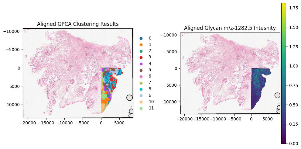
The manual alignment has worked very well. The MALDI pixels are correctly located in the bottom right section of the tissue. To visualise the before/after alignment changes we can exclude the term ‘aligned’ from the .pl.show() call. This will plot both the ‘aligned’ and original ‘global’ coordinate systems.
[20]:
aligned.pl.render_images("he_image") \
       .pl.render_shapes("pixels", color="MPI")\
       .pl.show()
INFO     Rasterizing image for faster rendering.
INFO     Using 'datashader' backend with 'None' as reduction method to speed up plotting. Depending on the
         reduction method, the value range of the plot might change. Set method to 'matplotlib' to disable this
         behaviour.
INFO     Using the datashader reduction "mean". "max" will give an output very close to the matplotlib result.
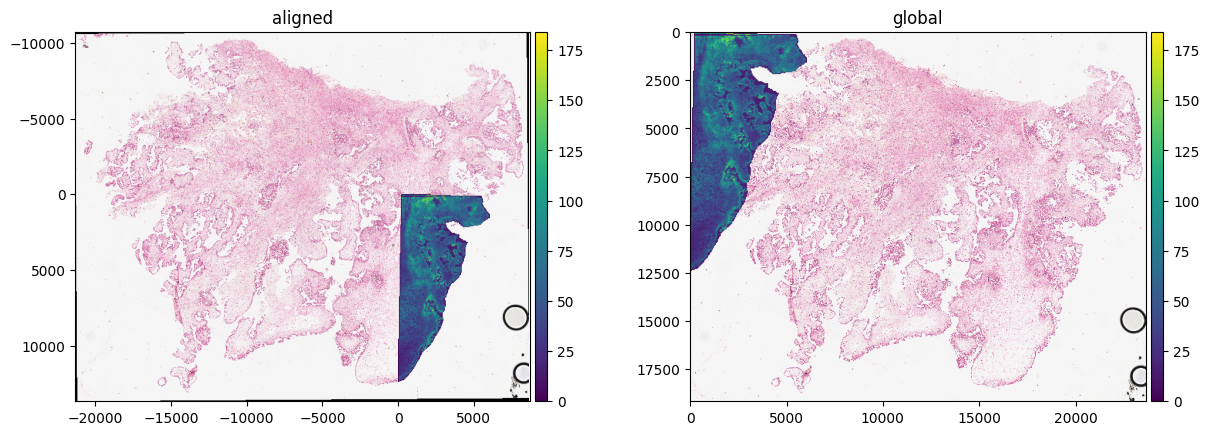
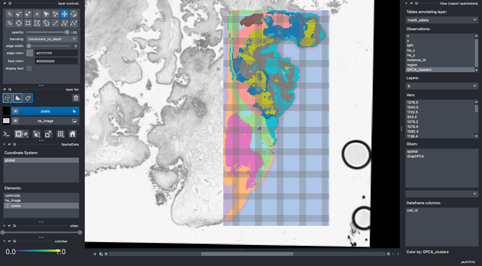
Based on these plots the alignment was succesfully performed. This alignment can also be visualised interactivally using the Interactive function from napari-spatialdata
[21]:
interactive = Interactive(aligned)
viewer = interactive.run()
2026-04-17 01:04:07.970 | WARNING  | napari_spatialdata._viewer:__init__:57 - Due to Shift-L being used as shortcut in napari, it is being deprecated and might not link a new layer to an existing SpatialData object in the viewer. Please use ⌘-L on MacOS or else Ctrl-L.
2026-04-17 01:04:17.747 | DEBUG    | napari_spatialdata._view:_on_layer_update:569 - Updating layer.
2026-04-17 01:04:17.749 | DEBUG    | napari_spatialdata._view:_on_layer_update:569 - Updating layer.
2026-04-17 01:04:23.356 | DEBUG    | napari_spatialdata._view:_on_layer_update:569 - Updating layer.
2026-04-17 01:04:23.374 | DEBUG    | napari_spatialdata._view:_on_layer_update:569 - Updating layer.
2026-04-17 01:04:23.501 | DEBUG    | napari_spatialdata._view:_on_layer_update:569 - Updating layer.
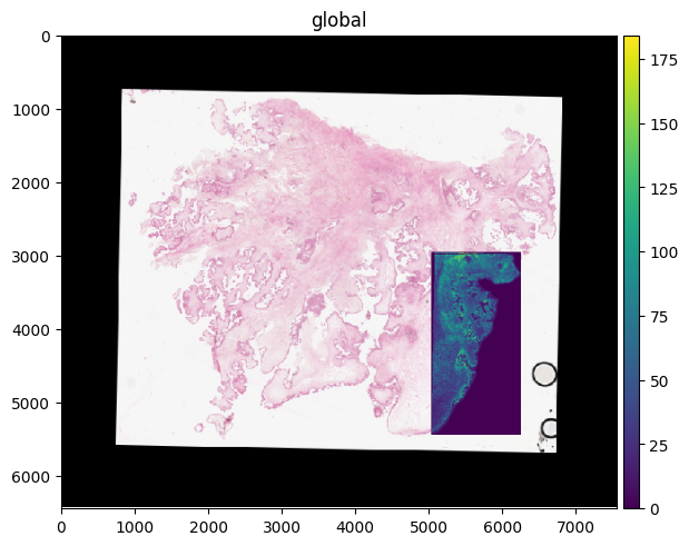
Automatic MALDI/H&E Alignment#
Based on the manual alignment method displayed above, we will use goatpy’s automated alignment method (gp.load_and_align) to acheive the same results.
[22]:
sdata = gp.load_and_align(imzml_path = "./Documents/AD_resolution_change_check_10um_actual_10012020_2.imzML",
                          he_path="./Documents/res_check_0000.tif")
[2.65GB]   Loading peaks ...
[2.65GB]   108 peaks
[2.62GB]   WARNING: H&E pixel size unknown, assuming 0.2527 um/px.
[2.52GB]   MALDI pixel size from imzML metadata: 400.0 um/px
[2.52GB]   WARNING: imzML pixel size 400.0 um makes H&E thumbnail (15x12 px) smaller than MALDI (2760x1126 px) -- likely wrong.
[2.52GB]   Falling back to maldi_pixel_um=10.0 um/px.
[2.52GB]   maldi_pixel_um=10.0  he_pixel_um=0.2527
[2.52GB]   Computing MALDI crop offsets ...
[0.45GB]   Crop: row=877, col=2638
[0.93GB]   Loading 108 ion images (chunk=10) ...
[0.20GB]   Peaks 1-10 / 108
[0.19GB]   Peaks 11-20 / 108
[0.20GB]   Peaks 21-30 / 108
[0.19GB]   Peaks 31-40 / 108
[0.19GB]   Peaks 41-50 / 108
[0.19GB]   Peaks 51-60 / 108
[0.20GB]   Peaks 61-70 / 108
[0.19GB]   Peaks 71-80 / 108
[0.21GB]   Peaks 81-90 / 108
[0.19GB]   Peaks 91-100 / 108
[0.23GB]   Peaks 101-108 / 108
[0.25GB]   spectra_all: (249, 122, 108)  (13 MB)
[0.25GB]   Preparing MALDI template ...
[0.25GB]   MALDI grayscale: (249, 122)  mean=0.204
[0.70GB]   Loading H&E at 10.0 um/px ...
[0.92GB]   PIL: 23633x19160
[0.32GB]   Resized to 597x484  10.000 um/px  (1 MB)
[0.32GB]   H&E: 597x484  (1 MB)
[0.32GB]   Preparing H&E search image ...
[0.32GB]   H&E grayscale: (484, 597)  mean=0.104
[0.32GB]   Running registration ...
[0.32GB]   Coarse: 24 rotations (0-360 step 15) ...
[0.34GB]       0.0  score=0.7926
[0.36GB]      15.0  score=0.5688
[0.38GB]      30.0  score=0.5883
[0.39GB]      45.0  score=0.5499
[0.39GB]      60.0  score=0.5186
[0.40GB]      75.0  score=0.5548
[0.40GB]      90.0  score=0.6474
[0.42GB]     105.0  score=0.6431
[0.43GB]     120.0  score=0.6185
[0.45GB]     135.0  score=0.6084
[0.45GB]     150.0  score=0.5942
[0.45GB]     165.0  score=0.5689
[0.45GB]     180.0  score=0.4967
[0.46GB]     195.0  score=0.6934
[0.47GB]     210.0  score=0.7018
[0.47GB]     225.0  score=0.6115
[0.47GB]     240.0  score=0.5855
[0.47GB]     255.0  score=0.5570
[0.47GB]     270.0  score=0.4412
[0.47GB]     285.0  score=0.5037
[0.48GB]     300.0  score=0.5393
[0.49GB]     315.0  score=0.5276
[0.50GB]     330.0  score=0.5203
[0.50GB]     345.0  score=0.5785
[0.50GB]   Best coarse: 0.0  score=0.7926
[0.50GB]   Fine: 10 rotations (+-5.0 step 1.0) ...
[0.50GB]      -5.0  score=0.6809
[0.50GB]      -4.0  score=0.6995
[0.50GB]      -3.0  score=0.7198
[0.50GB]      -2.0  score=0.7537
[0.50GB]      -1.0  score=0.7958
[0.51GB]       1.0  score=0.8036
[0.51GB]       2.0  score=0.7689
[0.51GB]       3.0  score=0.7381
[0.51GB]       4.0  score=0.7142
[0.51GB]       5.0  score=0.6999
[0.51GB]   Final: 1.0  score=0.8036  offset=(296, 503)
[1.09GB]   Building H&E output canvas ...
[1.09GB]   H&E canvas (cv2): 755x644  pr=75, pc=75  rotation=1.0
[1.09GB]   Building SpatialData ...
[1.39GB]   H&E upscaled 10x: 7550x6440  (146 MB)
[1.43GB]   Transform stored: rotation=1.0  he_reg_size=[484, 597]  canvas_placement=[75, 75]
[1.43GB]   Done.
Lets look at the data structure of our automatically aligned object. We can see it follows a very similar layout to the manual alignment method. One key difference is that unlike the aligned object using the manual alignment method all aligned data is stored in the global coordinate system, rather than the system named aligned.
[23]:
sdata
[23]:
SpatialData object
├── Images
│     └── 'he_image': DataArray[cyx] (3, 6440, 7550)
├── Points
│     └── 'centroids': DataFrame with shape: (<Delayed>, 3) (2D points)
├── Shapes
│     └── 'pixels': GeoDataFrame shape: (30378, 2) (2D shapes)
└── Tables
      └── 'maldi_adata': AnnData (30378, 108)
with coordinate systems:
    ▸ 'global', with elements:
        he_image (Images), centroids (Points), pixels (Shapes)
We can check if the automatic alignment was successfull by plotting the MPI intesnity values.
[24]:
sdata.pl.render_images("he_image") \
     .pl.render_shapes("pixels", color="MPI") \
     .pl.show()
INFO     Rasterizing image for faster rendering.
INFO     Using 'datashader' backend with 'None' as reduction method to speed up plotting. Depending on the
         reduction method, the value range of the plot might change. Set method to 'matplotlib' to disable this
         behaviour.
INFO     Using the datashader reduction "mean". "max" will give an output very close to the matplotlib result.
Now that our data is correctly aligned we can run more downstream analyses such as clustering.
[25]:
sdata = gp.graphpca_spatialdata(sdata, tables= "maldi_adata",
    library_id= 'spatial',
    n_components = 50,
    n_neighbors = 15,
    alpha = 0.5)

sdata = gp.get_kmean_clusters(sdata, tables= "maldi_adata",n_clusters = 12)
[26]:
sdata.pl.render_images("he_image") \
     .pl.render_shapes("pixels", color="GPCA_clusters") \
     .pl.show()
INFO     Rasterizing image for faster rendering.
INFO     Using 'datashader' backend with 'None' as reduction method to speed up plotting. Depending on the
         reduction method, the value range of the plot might change. Set method to 'matplotlib' to disable this
         behaviour.
Again we can also use napari-spatialdata to visualise these results.
[27]:
interactive = Interactive(sdata)
viewer = interactive.run()
2026-04-17 19:48:44.444 | WARNING | napari_spatialdata._viewer:__init__:57 - Due to Shift-L being used as shortcut in napari, it is being deprecated and might not link a new layer to an existing SpatialData object in the viewer. Please use ⌘-L on MacOS or else Ctrl-L.
2026-04-17 19:48:49.032 | DEBUG    | napari_spatialdata._view:_on_layer_update:569 - Updating layer.
2026-04-17 19:48:49.033 | DEBUG    | napari_spatialdata._view:_on_layer_update:569 - Updating layer.
2026-04-17 19:48:55.213 | DEBUG    | napari_spatialdata._view:_on_layer_update:569 - Updating layer.
2026-04-17 19:48:55.237 | DEBUG    | napari_spatialdata._view:_on_layer_update:569 - Updating layer.
2026-04-17 19:48:55.284 | DEBUG    | napari_spatialdata._view:_on_layer_update:569 - Updating layer.
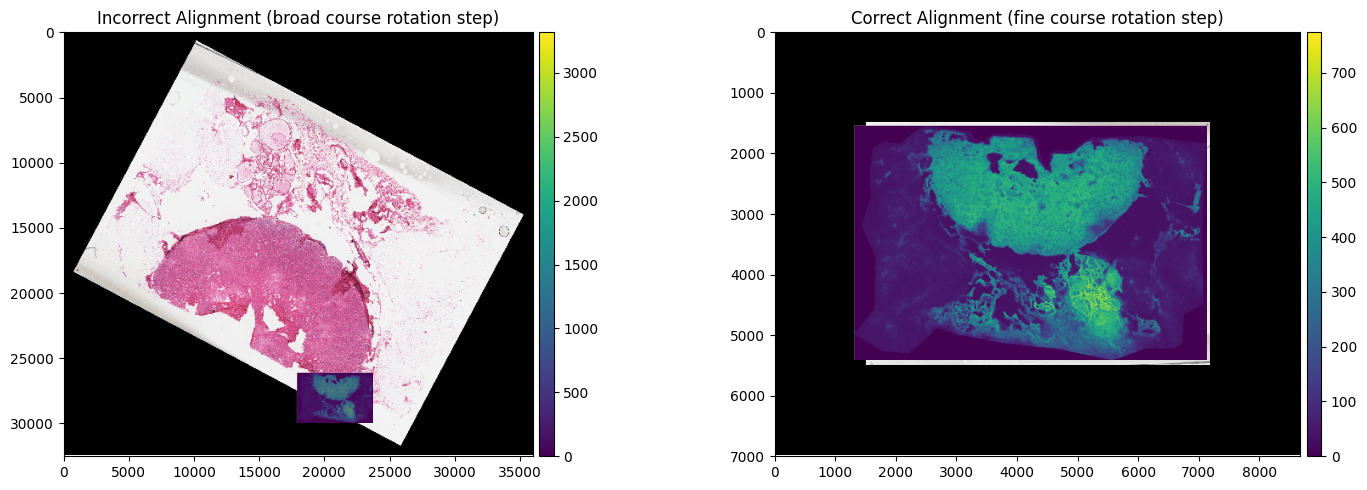
There will be some cases where the inital run of autoalignment using the default parameters doesnt exactly work.
Some common reasons for this include:
incorrect/unspecified maldi pixel size (
maldi_pixel_um) extracted from .imzML/.ibd fileunspecified H&E image pixel size (
he_pixel_um) when using a.TIFF/.TIFimage rather than a.svsfilecoarse rotation step needs a finer search (
coarse_rotation_steprequires a lower value)
It is possible that other parameters may need adjustment, and it is recomended to change these accordinly depeneding on the data.
[28]:
unaligned_dataset = gp.load_and_align(imzml_path = "./Documents/breast_cancer_concr_0022/concr_tnbc_0022-s2-total_ion_count.imzML",
                        peaks_path = "./Documents/breast_cancer_concr_0022/breast_peaks_formatted.csv",
                        he_path="./Documents/breast_cancer_concr_0022/tnbc_0022.svs")
[0.22GB]   Loading peaks ...
[0.22GB]   121 peaks
[0.23GB]   H&E native pixel size: 0.2527 um/px
[0.29GB]   MALDI pixel size from imzML metadata: 50.0 um/px
[0.30GB]   WARNING: imzML pixel size 50.0 um makes H&E thumbnail (568x401 px) smaller than MALDI (582x386 px) -- likely wrong.
[0.30GB]   Auto-selected maldi_pixel_um=10.0 um/px
[0.30GB]   maldi_pixel_um=10.0  he_pixel_um=0.2527
[0.30GB]   Computing MALDI crop offsets ...
[0.56GB]   Crop: row=0, col=0
[0.56GB]   Loading 121 ion images (chunk=10) ...
[0.16GB]   Peaks 1-10 / 121
[0.15GB]   Peaks 11-20 / 121
[0.16GB]   Peaks 21-30 / 121
[0.16GB]   Peaks 31-40 / 121
[0.16GB]   Peaks 41-50 / 121
[0.16GB]   Peaks 51-60 / 121
[0.16GB]   Peaks 61-70 / 121
[0.16GB]   Peaks 71-80 / 121
[0.16GB]   Peaks 81-90 / 121
[0.16GB]   Peaks 91-100 / 121
[0.15GB]   Peaks 101-110 / 121
[0.16GB]   Peaks 111-120 / 121
[0.27GB]   Peaks 121-121 / 121
[0.29GB]   spectra_all: (386, 582, 121)  (109 MB)
[0.29GB]   Preparing MALDI template ...
[0.29GB]   MALDI grayscale: (386, 582)  mean=0.235
[0.70GB]   Loading H&E at 10.0 um/px ...
[0.79GB]   openslide level 3: 3510x2479  8.087 um/px  (26 MB)
[0.72GB]   Resized to 2839x2005  10.000 um/px
[0.72GB]   H&E: 2839x2005  (17 MB)
[0.72GB]   Preparing H&E search image ...
[0.77GB]   H&E grayscale: (2005, 2839)  mean=0.189
[0.79GB]   Running registration ...
[0.79GB]   Coarse: 24 rotations (0-360 step 15) ...
[0.87GB]       0.0  score=0.3997
[1.09GB]      15.0  score=0.4535
[1.27GB]      30.0  score=0.4984
[1.38GB]      45.0  score=0.4949
[1.39GB]      60.0  score=0.4344
[1.40GB]      75.0  score=0.4096
[1.41GB]      90.0  score=0.3769
[1.40GB]     105.0  score=0.3543
[1.41GB]     120.0  score=0.3350
[1.41GB]     135.0  score=0.3708
[1.41GB]     150.0  score=0.3971
[1.41GB]     165.0  score=0.4499
[1.43GB]     180.0  score=0.4272
[1.43GB]     195.0  score=0.4150
[1.43GB]     210.0  score=0.4233
[1.43GB]     225.0  score=0.4050
[1.43GB]     240.0  score=0.4398
[1.43GB]     255.0  score=0.4926
[1.43GB]     270.0  score=0.4708
[1.43GB]     285.0  score=0.4588
[1.43GB]     300.0  score=0.4557
[1.43GB]     315.0  score=0.4756
[1.43GB]     330.0  score=0.4892
[1.43GB]     345.0  score=0.4399
[1.43GB]   Best coarse: 30.0  score=0.4984
[1.43GB]   Fine: 10 rotations (+-5.0 step 1.0) ...
[1.44GB]      25.0  score=0.4938
[1.44GB]      26.0  score=0.4976
[1.44GB]      27.0  score=0.4994
[1.44GB]      28.0  score=0.5008
[1.44GB]      29.0  score=0.5004
[1.44GB]      31.0  score=0.4955
[1.44GB]      32.0  score=0.4920
[1.44GB]      33.0  score=0.4875
[1.44GB]      34.0  score=0.4810
[1.44GB]      35.0  score=0.4743
[1.44GB]   Final: 28.0  score=0.5008  offset=(2611, 1785)
[1.44GB]   Building H&E output canvas ...
[1.46GB]   H&E canvas (cv2): 3597x3252  pr=75, pc=75  rotation=28.0
[1.46GB]   Transforming annotations: /Users/andrewcauser/Documents/Griffith/test_data/breast_cancer_concr_0022/tnbc_0022_annotations.geojson ...
[1.47GB]   17 annotations  |  classes: ['Tumor', 'Fibroblasts', 'Region*', 'Adipose', 'Immune cells', 'Stroma', 'Ducts']
[1.47GB]   Building SpatialData ...
[0.37GB]   H&E upscaled 10x: 35970x32520  (3509 MB)
[4.44GB]   Annotations added -> sdata.shapes['annotations']
[4.44GB]   Transform stored: rotation=28.0  he_reg_size=[2005, 2839]  canvas_placement=[75, 75]
[4.44GB]   Done.
[29]:
aligned_dataset = gp.load_and_align(imzml_path = "./Documents/breast_cancer_concr_0022/concr_tnbc_0022-s2-total_ion_count.imzML",
                        peaks_path = "./Documents/breast_cancer_concr_0022/breast_peaks_formatted.csv",
                        he_path="./Documents/breast_cancer_concr_0022/tnbc_0022.svs",
                        maldi_pixel_um=50,
                        coarse_rotation_step=5,   # finer search — more likely to find correct angle
                        buffer_px=300)
[0.33GB]   Loading peaks ...
[0.33GB]   121 peaks
[0.34GB]   H&E native pixel size: 0.2527 um/px
[0.34GB]   MALDI pixel size (supplied): 50 um/px
[0.34GB]   maldi_pixel_um=50  he_pixel_um=0.2527
[0.34GB]   Computing MALDI crop offsets ...
[0.58GB]   Crop: row=0, col=0
[0.58GB]   Loading 121 ion images (chunk=10) ...
[0.16GB]   Peaks 1-10 / 121
[0.17GB]   Peaks 11-20 / 121
[0.16GB]   Peaks 21-30 / 121
[0.16GB]   Peaks 31-40 / 121
[0.16GB]   Peaks 41-50 / 121
[0.16GB]   Peaks 51-60 / 121
[0.16GB]   Peaks 61-70 / 121
[0.16GB]   Peaks 71-80 / 121
[0.18GB]   Peaks 81-90 / 121
[0.16GB]   Peaks 91-100 / 121
[0.16GB]   Peaks 101-110 / 121
[0.16GB]   Peaks 111-120 / 121
[0.25GB]   Peaks 121-121 / 121
[0.27GB]   spectra_all: (386, 582, 121)  (109 MB)
[0.27GB]   Preparing MALDI template ...
[0.27GB]   MALDI grayscale: (386, 582)  mean=0.235
[0.69GB]   Loading H&E at 50 um/px ...
[0.78GB]   openslide level 3: 3510x2479  8.087 um/px  (26 MB)
[0.78GB]   Resized to 568x401  50.000 um/px
[0.78GB]   H&E: 568x401  (1 MB)
[0.78GB]   Preparing H&E search image ...
[0.78GB]   H&E grayscale: (401, 568)  mean=0.218
[0.78GB]   Running registration ...
[0.78GB]   Coarse: 72 rotations (0-360 step 5) ...
[0.79GB]       0.0  score=0.4617
[0.80GB]       5.0  score=0.4777
[0.81GB]      10.0  score=0.4951
[0.83GB]      15.0  score=0.5171
[0.84GB]      20.0  score=0.5431
[0.85GB]      25.0  score=0.5633
[0.86GB]      30.0  score=0.5893
[0.88GB]      35.0  score=0.6009
[0.90GB]      40.0  score=0.5984
[0.91GB]      45.0  score=0.5920
[0.92GB]      50.0  score=0.5863
[0.92GB]      55.0  score=0.5895
[0.94GB]      60.0  score=0.5846
[0.94GB]      65.0  score=0.5741
[0.94GB]      70.0  score=0.5498
[0.94GB]      75.0  score=0.5178
[0.94GB]      80.0  score=0.4802
[0.94GB]      85.0  score=0.4424
[0.94GB]      90.0  score=0.4156
[0.94GB]      95.0  score=0.4158
[0.94GB]     100.0  score=0.4180
[0.94GB]     105.0  score=0.4217
[0.94GB]     110.0  score=0.4154
[0.94GB]     115.0  score=0.4325
[0.94GB]     120.0  score=0.4525
[0.94GB]     125.0  score=0.4833
[0.94GB]     130.0  score=0.5154
[0.94GB]     135.0  score=0.5461
[0.95GB]     140.0  score=0.5717
[0.95GB]     145.0  score=0.5875
[0.96GB]     150.0  score=0.5994
[0.96GB]     155.0  score=0.6101
[0.96GB]     160.0  score=0.6247
[0.96GB]     165.0  score=0.6487
[0.96GB]     170.0  score=0.6870
[0.96GB]     175.0  score=0.7167
[0.96GB]     180.0  score=0.8093
[0.97GB]     185.0  score=0.7060
[0.97GB]     190.0  score=0.6744
[0.97GB]     195.0  score=0.6369
[0.97GB]     200.0  score=0.6045
[0.97GB]     205.0  score=0.5702
[0.97GB]     210.0  score=0.5481
[0.97GB]     215.0  score=0.5238
[0.97GB]     220.0  score=0.5056
[0.97GB]     225.0  score=0.4796
[0.97GB]     230.0  score=0.4534
[0.97GB]     235.0  score=0.4306
[0.97GB]     240.0  score=0.4319
[0.97GB]     245.0  score=0.4441
[0.97GB]     250.0  score=0.4632
[0.97GB]     255.0  score=0.4853
[0.97GB]     260.0  score=0.5235
[0.97GB]     265.0  score=0.5539
[0.97GB]     270.0  score=0.5612
[0.97GB]     275.0  score=0.5689
[0.97GB]     280.0  score=0.5581
[0.97GB]     285.0  score=0.5348
[0.97GB]     290.0  score=0.5187
[0.97GB]     295.0  score=0.5001
[0.97GB]     300.0  score=0.4853
[0.97GB]     305.0  score=0.4709
[0.97GB]     310.0  score=0.4577
[0.97GB]     315.0  score=0.4421
[0.97GB]     320.0  score=0.4211
[0.97GB]     325.0  score=0.4241
[0.97GB]     330.0  score=0.4340
[0.97GB]     335.0  score=0.4435
[0.97GB]     340.0  score=0.4456
[0.97GB]     345.0  score=0.4473
[0.97GB]     350.0  score=0.4534
[0.97GB]     355.0  score=0.4561
[0.97GB]   Best coarse: 180.0  score=0.8093
[0.97GB]   Fine: 10 rotations (+-5.0 step 1.0) ...
[0.97GB]     175.0  score=0.7167
[0.97GB]     176.0  score=0.7257
[0.97GB]     177.0  score=0.7387
[0.97GB]     178.0  score=0.7577
[0.97GB]     179.0  score=0.7864
[0.97GB]     181.0  score=0.7835
[0.97GB]     182.0  score=0.7486
[0.97GB]     183.0  score=0.7308
[0.97GB]     184.0  score=0.7174
[0.97GB]     185.0  score=0.7060
[0.97GB]   Final: 180.0  score=0.8093  offset=(156, 131)
[0.97GB]   Building H&E output canvas ...
[0.97GB]   H&E canvas (cv2): 867x700  pr=150, pc=150  rotation=180.0
[0.97GB]   Building SpatialData ...
[1.32GB]   H&E upscaled 10x: 8670x7000  (182 MB)
[1.33GB]   Transform stored: rotation=180.0  he_reg_size=[401, 568]  canvas_placement=[150, 150]
[1.33GB]   Done.
[30]:
fig, axes = plt.subplots(1, 2, figsize=(15, 5))

unaligned_dataset.pl.render_images("he_image") \
     .pl.render_shapes("pixels", color="MPI") \
     .pl.show(ax=axes[0], title="Incorrect Alignment (broad course rotation step)")

aligned_dataset.pl.render_images("he_image") \
     .pl.render_shapes("pixels", color="MPI") \
     .pl.show(ax=axes[1], title="Correct Alignment (fine course rotation step)")


plt.tight_layout()
plt.show()
INFO     Rasterizing image for faster rendering.
INFO     Using 'datashader' backend with 'None' as reduction method to speed up plotting. Depending on the
         reduction method, the value range of the plot might change. Set method to 'matplotlib' to disable this
         behaviour.
INFO     Using the datashader reduction "mean". "max" will give an output very close to the matplotlib result.
Loading with specific m/z values#
goatpy allows the user to provide a list of m/z values to use for importing the data, in the form of a .csv file. If no file is specified peaks will be imported using a default peak list. Below is an example of how to import data using either the gp.load_and_align or glyco_spatialdata.
[31]:
path = "./Documents/breast_cancer_concr_0019/concr_tnbc_0019-s1-total_ion_count.imzML"
peaks = "./Documents/breast_cancer_concr_0019/breast_peaks_formatted.csv"

## Using manual alignment function
sdata = gp.glyco_spatialdata(imzml_path=path, peaks_path=peaks)

## Using automatic alignment function
auto_align = gp.load_and_align(imzml_path = path,
                               peaks_path = peaks,
                               he_path="./Documents/breast_cancer_concr_0019/tnbc_0019.svs")
Adding Pathologist annotations#
Along with aligning a H&E image to your MALDI glycomics data, you can also add pathology or regional tissue annotations to a goatpy SpatialData object. Below we will demonstrate how to do this for either the manual or automated alignment methods described above.
Currently goatpy handels patholigst annotations exported from QuPath in the form of .geojson files. These annotations must be generated/corresponding to the exact same file imported into either gp.he_spatialdata or gp.load_and_align.
To export the annotations in QuPath go to: file → Export objects as GeoJSON → Select Export as FeatureCollection → OK. The exported .GeoJSON file should have atleast 2 columns called ‘classification’ and ‘geometry’. An example is displayed below:
classification    {'name': 'Fibroblasts', 'color': [250, 194, 194]}
geometry          POLYGON ((22746 16005, 22745.67 16005.22, 2274...
Adding Annotations Using Manual Alignment#
Below is an example of how to add pathology annotations when using the manual alignment functionality of •goatpy•. First we must create our SpatialData object for our H&E image.
[32]:
he_path = "./Documents/breast_cancer_concr_0019/tnbc_0019.svs"
example_he = gp.he_spatialdata(he_path)
Successfully loaded with sopa.io.wsi
Once loaded we can then add the annotations from the .geojson file to our spaitaldata object, and then visualise the annotations plotted over the H&E to check they match.
[33]:
example_he = gp.add_annotations(example_he, geojson_path = "./Downloads/breast_cancer_concr_0019/tnbc_0019.geojson")
[34]:
example_he.pl.render_images("he_image")\
       .pl.render_shapes("Annotations", color="classification")\
       .pl.show()
INFO Rasterizing image for faster rendering.
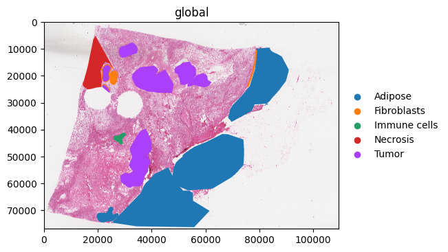
We can see that our data overlays well and we are ready to continue with the alignment of MALDI pixel data to the H&E image. These steps are the same as those discribed above.
[35]:
## Load MALDI data
path = "./Documents/breast_cancer_concr_0019/concr_tnbc_0019-s1-total_ion_count.imzML"
sdata = gp.glyco_spatialdata(imzml_path=path, peaks_path="./Documents/breast_cancer_concr_0019/breast_peaks_formatted.csv")

## Add Psuedo-Image
sdata = gp.Add_Pseudo_Image(sdata, "MPI", tables = "maldi_adata", library_id = "Spatial", is_continous=True, cmap = "viridis",img_upscaling=50)
INFO Transposing `data` of type: <class 'dask.array.core.Array'> to ('c', 'y', 'x').
[36]:
## Run Manual Alignment
viewer, widget = gp.launch_landmark_gui(sdata, example_he, split_view=False, he_scale_level="scale1")
Available MALDI scale levels:
  scale0: (3, 18900, 27100)
  scale1: (3, 9450, 13550)
  scale2: (3, 4725, 6775)
  scale3: (3, 2362, 3387)
Available H&E scale levels:
  scale0: (3, 76899, 109479)
  scale1: (3, 19224, 27369)
  scale2: (3, 4806, 6842)
  scale3: (3, 2403, 3421)

No maldi_scale_level specified — defaulting to 'scale0'.

Launching GUI with MALDI=scale0, H&E=scale1
[LandmarkGUI] MALDI display level=scale0, scale_factor=1.000  |  H&E display level=scale1, scale_factor=4.000
ValueError: All border_width must be between 0 and 1 if border_width_is_relative is enabled
INFO: Saved 5 landmark pairs (scaled to full resolution)
INFO: Saved 5 landmark pairs (scaled to full resolution)
[37]:
sdata["maldi_landmarks"].compute()
[37]:
| x | y | |
|---|---|---|
| 0 | 26887.388227 | 1681.706517 |
| 1 | 11642.543891 | 1073.534536 |
| 2 | 7993.512002 | 4763.111223 |
| 3 | 19143.331663 | 11453.003020 |
| 4 | 22224.736369 | 12182.809398 |
[38]:
aligned = gp.align_image_using_landmarks(sdata, example_he)
[39]:
aligned["centroids"]
[39]:
| x | y | instance_id | region | mz-1298.6 | mz-1257.6 | mz-1339.6 | mz-1401.6 | mz-1419.7 | mz-1444.7 | mz-1460.7 | mz-1485.7 | mz-1501.7 | mz-1524.7 | mz-1542.7 | mz-1546.7 | mz-1563.7 | mz-1581.7 | mz-1602.8 | mz-1611.7 | mz-1622.7 | mz-1629.8 | mz-1647.8 | mz-1663.8 | mz-1675.8 | mz-1679.7 | mz-1688.8 | mz-1704.8 | mz-1708.8 | mz-1725.8 | mz-1743.8 | mz-1748.9 | mz-1764.8 | mz-1791.8 | mz-1784.9 | mz-1809.8 | mz-1820.9 | mz-1825.8 | mz-1828.8 | mz-1837.8 | mz-1850.9 | mz-1866.9 | mz-1891.9 | mz-1905.8 | mz-1910.9 | mz-1926.9 | mz-1951.9 | mz-1955.9 | mz-1967.9 | mz-1976.9 | mz-1983.9 | mz-1994.9 | mz-2012.9 | mz-1998.9 | mz-2028.9 | mz-2057.0 | mz-2067.9 | mz-2114.0 | mz-2122.9 | mz-2101.9 | mz-2095.9 | mz-2129.9 | mz-2133.0 | mz-2142.0 | mz-2155.0 | mz-2171.0 | mz-2174.9 | mz-2216.0 | mz-2260.0 | mz-2272.0 | mz-2281.0 | mz-2303.0 | mz-2317.0 | mz-2321.0 | mz-2326.1 | mz-2333.0 | mz-2377.9 | mz-2394.0 | mz-2418.0 | mz-2449.1 | mz-2427.0 | mz-2467.0 | mz-2479.0 | mz-2540.0 | mz-2620.9 | mz-2637.1 | mz-2771.0 | mz-2905.9 | mz-2941.8 | mz-3087.8 | mz-3209.6 | mz-933.5 | mz-1095.6 | mz-1136.6 | mz-1239.6 | mz-2487.9 | mz-2520.0 | mz-2645.9 | mz-2682.0 | mz-2743.0 | mz-2758.9 | mz-2928.8 | mz-3148.7 | mz-3270.5 | mz-2990.8 | mz-3063.8 | mz-1079.4 | mz-1278.5 | mz-1282.8 | mz-2052.1 | mz-2342.2 | mz-2698.4 | mz-2687.4 | mz-2784.4 | mz-2844.4 | mz-2793.4 | mz-2855.5 | mz-3002.6 | mz-3052.5 | mz-3137.6 | mz-3198.5 | mz-3283.5 | mz-3295.5 | mz-3307.5 | mz-3356.6 | |
|---|---|---|---|---|---|---|---|---|---|---|---|---|---|---|---|---|---|---|---|---|---|---|---|---|---|---|---|---|---|---|---|---|---|---|---|---|---|---|---|---|---|---|---|---|---|---|---|---|---|---|---|---|---|---|---|---|---|---|---|---|---|---|---|---|---|---|---|---|---|---|---|---|---|---|---|---|---|---|---|---|---|---|---|---|---|---|---|---|---|---|---|---|---|---|---|---|---|---|---|---|---|---|---|---|---|---|---|---|---|---|---|---|---|---|---|---|---|---|---|---|---|---|---|---|---|
| npartitions=1 | |||||||||||||||||||||||||||||||||||||||||||||||||||||||||||||||||||||||||||||||||||||||||||||||||||||||||||||||||||||||||||||
| 0 | int64 | int64 | string | string | float32 | float32 | float32 | float32 | float32 | float32 | float32 | float32 | float32 | float32 | float32 | float32 | float32 | float32 | float32 | float32 | float32 | float32 | float32 | float32 | float32 | float32 | float32 | float32 | float32 | float32 | float32 | float32 | float32 | float32 | float32 | float32 | float32 | float32 | float32 | float32 | float32 | float32 | float32 | float32 | float32 | float32 | float32 | float32 | float32 | float32 | float32 | float32 | float32 | float32 | float32 | float32 | float32 | float32 | float32 | float32 | float32 | float32 | float32 | float32 | float32 | float32 | float32 | float32 | float32 | float32 | float32 | float32 | float32 | float32 | float32 | float32 | float32 | float32 | float32 | float32 | float32 | float32 | float32 | float32 | float32 | float32 | float32 | float32 | float32 | float32 | float32 | float32 | float32 | float32 | float32 | float32 | float32 | float32 | float32 | float32 | float32 | float32 | float32 | float32 | float32 | float32 | float32 | float32 | float32 | float32 | float32 | float32 | float32 | float32 | float32 | float32 | float32 | float32 | float32 | float32 | float32 | float32 | float32 | float32 | float32 |
| 137854 | ... | ... | ... | ... | ... | ... | ... | ... | ... | ... | ... | ... | ... | ... | ... | ... | ... | ... | ... | ... | ... | ... | ... | ... | ... | ... | ... | ... | ... | ... | ... | ... | ... | ... | ... | ... | ... | ... | ... | ... | ... | ... | ... | ... | ... | ... | ... | ... | ... | ... | ... | ... | ... | ... | ... | ... | ... | ... | ... | ... | ... | ... | ... | ... | ... | ... | ... | ... | ... | ... | ... | ... | ... | ... | ... | ... | ... | ... | ... | ... | ... | ... | ... | ... | ... | ... | ... | ... | ... | ... | ... | ... | ... | ... | ... | ... | ... | ... | ... | ... | ... | ... | ... | ... | ... | ... | ... | ... | ... | ... | ... | ... | ... | ... | ... | ... | ... | ... | ... | ... | ... | ... | ... | ... | ... |
[40]:
fig, axes = plt.subplots(1, 2, figsize=(20, 5))

aligned.pl.render_images("he_image")\
    .pl.render_points("centroids",size = 8,color="mz-1339.6", alpha = 0)\
    .pl.render_shapes("Annotations",color="classification", fill_alpha = 0.5)\
    .pl.show("aligned", ax=axes[0], title="Aligned Pathology annotation with H&E")

aligned.pl.render_images("he_image")\
    .pl.render_points("centroids",size = 8,color="mz-1339.6")\
    .pl.render_shapes("Annotations",color="classification", fill_alpha = 0.5)\
    .pl.show("aligned", ax=axes[1], title="Aligned Pathology annotation with Glycan m/z-1339.6")

plt.tight_layout()
plt.show()
INFO     Rasterizing image for faster rendering.
INFO     Using 'datashader' backend with 'None' as reduction method to speed up plotting. Depending on the
         reduction method, the value range of the plot might change. Set method to 'matplotlib' do disable this
         behaviour.
INFO     Using the datashader reduction "sum". "max" will give an output very close to the matplotlib result.
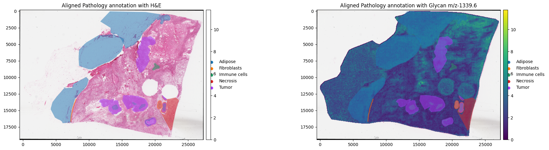
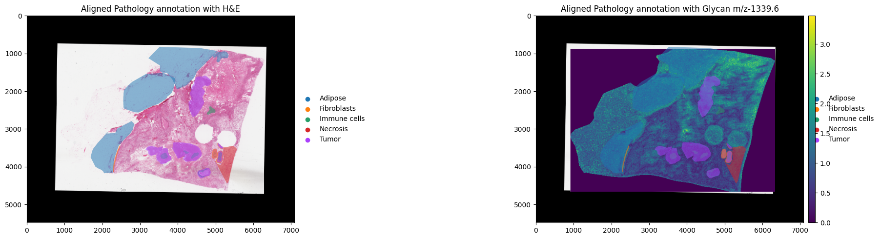
Adding Annotations Using Automatic Alignment#
Pathology annotations can also be added using the automatic alignment approach. Using the same example we will use the gp.load_and_align function to demonstrate this:
[41]:
sdata = gp.load_and_align(imzml_path = "./Documents/breast_cancer_concr_0019/concr_tnbc_0019-s1-total_ion_count.imzML",
                        peaks_path = "./Documents/breast_cancer_concr_0019/breast_peaks_formatted.csv",
                        he_path="./Documents/breast_cancer_concr_0019/tnbc_0019.svs",
                        geojson_path = "./Documents/breast_cancer_concr_0019/tnbc_0019_annotations.geojson",
                        )
[0.08GB]   Loading peaks ...
[0.09GB]   121 peaks
[0.10GB]   H&E native pixel size: 0.2527 um/px
[0.16GB]   MALDI pixel size from imzML metadata: 50.0 um/px
[0.13GB]   Validated: H&E thumbnail (553x389 px) >= MALDI (542x378 px)
[0.13GB]   maldi_pixel_um=50.0  he_pixel_um=0.2527
[0.13GB]   Computing MALDI crop offsets ...
[0.19GB]   Crop: row=0, col=0
[0.84GB]   Loading 121 ion images (chunk=10) ...
[0.16GB]   Peaks 1-10 / 121
[0.16GB]   Peaks 11-20 / 121
[0.16GB]   Peaks 21-30 / 121
[0.16GB]   Peaks 31-40 / 121
[0.16GB]   Peaks 41-50 / 121
[0.15GB]   Peaks 51-60 / 121
[0.15GB]   Peaks 61-70 / 121
[0.16GB]   Peaks 71-80 / 121
[0.15GB]   Peaks 81-90 / 121
[0.15GB]   Peaks 91-100 / 121
[0.15GB]   Peaks 101-110 / 121
[0.15GB]   Peaks 111-120 / 121
[0.20GB]   Peaks 121-121 / 121
[0.23GB]   spectra_all: (378, 542, 121)  (99 MB)
[0.24GB]   Preparing MALDI template ...
[0.24GB]   MALDI grayscale: (378, 542)  mean=0.174
[0.89GB]   Loading H&E at 50.0 um/px ...
[0.98GB]   openslide level 3: 3421x2403  8.087 um/px  (25 MB)
[0.99GB]   Resized to 553x389  50.000 um/px
[0.99GB]   H&E: 553x389  (1 MB)
[0.99GB]   Preparing H&E search image ...
[0.99GB]   H&E grayscale: (389, 553)  mean=0.189
[0.99GB]   Running registration ...
[0.99GB]   Coarse: 24 rotations (0-360 step 15) ...
[1.00GB]       0.0  score=0.3700
[1.02GB]      15.0  score=0.5223
[1.03GB]      30.0  score=0.5351
[1.04GB]      45.0  score=0.5118
[1.06GB]      60.0  score=0.4460
[1.06GB]      75.0  score=0.4410
[1.06GB]      90.0  score=0.2877
[1.06GB]     105.0  score=0.6163
[1.07GB]     120.0  score=0.6304
[1.07GB]     135.0  score=0.6176
[1.07GB]     150.0  score=0.6052
[1.07GB]     165.0  score=0.5890
[1.07GB]     180.0  score=0.6410
[1.07GB]     195.0  score=0.6079
[1.07GB]     210.0  score=0.5700
[1.08GB]     225.0  score=0.5486
[1.08GB]     240.0  score=0.5772
[1.08GB]     255.0  score=0.4813
[1.08GB]     270.0  score=0.2060
[1.08GB]     285.0  score=0.3448
[1.08GB]     300.0  score=0.4007
[1.08GB]     315.0  score=0.4336
[1.09GB]     330.0  score=0.4416
[1.09GB]     345.0  score=0.4183
[1.09GB]   Best coarse: 180.0  score=0.6410
[1.09GB]   Fine: 10 rotations (+-5.0 step 1.0) ...
[1.09GB]     175.0  score=0.6058
[1.09GB]     176.0  score=0.6111
[1.09GB]     177.0  score=0.6181
[1.09GB]     178.0  score=0.6290
[1.09GB]     179.0  score=0.6409
[1.09GB]     181.0  score=0.6455
[1.09GB]     182.0  score=0.6390
[1.09GB]     183.0  score=0.6341
[1.09GB]     184.0  score=0.6308
[1.09GB]     185.0  score=0.6298
[1.09GB]   Final: 181.0  score=0.6455  offset=(88, 91)
[1.09GB]   Building H&E output canvas ...
[1.09GB]   H&E canvas (cv2): 709x548  pr=75, pc=75  rotation=181.0
[1.09GB]   Transforming annotations: /Users/andrewcauser/Documents/Griffith/test_data/breast_cancer_concr_0019/tnbc_0019_annotations.geojson ...
[1.09GB]   24 annotations  |  classes: ['Necrosis', 'Fibroblasts', 'Immune cells', 'Tumor', 'Adipose']
[1.09GB]   Building SpatialData ...
[1.51GB]   H&E upscaled 10x: 7090x5480  (117 MB)
[1.30GB]   Annotations added -> sdata.shapes['annotations']
[1.30GB]   Transform stored: rotation=181.0  he_reg_size=[389, 553]  canvas_placement=[75, 75]
[1.30GB]   Done.
[42]:
fig, axes = plt.subplots(1, 2, figsize=(20, 5))

sdata.pl.render_images("he_image")\
    .pl.render_points("centroids",size = 8,color="mz-1339.6", alpha = 0)\
    .pl.render_shapes("annotations",color="classification", fill_alpha = 0.5)\
    .pl.show(ax=axes[0], title="Aligned Pathology annotation with H&E")

sdata.pl.render_images("he_image")\
    .pl.render_shapes("pixels",color="1339.6")\
     .pl.render_shapes("annotations",color="classification", fill_alpha = 0.5)\
    .pl.show(ax=axes[1], title="Aligned Pathology annotation with Glycan m/z-1339.6")

plt.tight_layout()
plt.show()
INFO     Rasterizing image for faster rendering.
INFO     Using 'datashader' backend with 'None' as reduction method to speed up plotting. Depending on the
         reduction method, the value range of the plot might change. Set method to 'matplotlib' do disable this
         behaviour.
INFO     Rasterizing image for faster rendering.
INFO     Using 'datashader' backend with 'None' as reduction method to speed up plotting. Depending on the
         reduction method, the value range of the plot might change. Set method to 'matplotlib' to disable this
         behaviour.
INFO     Using the datashader reduction "mean". "max" will give an output very close to the matplotlib result.
Assigning Annotations to the Pixel Level#
One the pathology annotations are aligned and stored in the SpatialData object, these annotations can be used to generate pixel level annotations based on overlapping regions. This is useful for performing downstream analyses and differential abundance analysis. We can use the gp.annotations_to_pixels function to do this. This function also takes in a parameter named overlap which lets the user specify the percentage of overlap required between the pixel and the respecitive polygon
for the pixel to be annotated.
[ ]:
sdata = gp.annotations_to_pixels(sdata)
    polygon_query 'Necrosis': 2,755 pixels
    polygon_query 'Fibroblasts': 805 pixels
    polygon_query 'Immune cells': 1,403 pixels
    polygon_query 'Tumor': 10,035 pixels
    polygon_query 'Adipose': 28,997 pixels
  [annotate_pixels] 'annotation' added: 42,721 / 204,876 pixels annotated  (20.9%)
    'other'                       :  162,155  (79.1%)
    'Necrosis'                    :    2,733  (1.3%)
    'Fibroblasts'                 :      470  (0.2%)
    'Immune cells'                :      486  (0.2%)
    'Tumor'                       :   10,035  (4.9%)
    'Adipose'                     :   28,997  (14.2%)
These results will be stored in the annotation column in the sdata["maldi_adata"].obs slot.
[44]:
sdata["maldi_adata"].obs
[44]:
| x | y | MPI | he_x | he_y | instance_id | region | annotation | |
|---|---|---|---|---|---|---|---|---|
| 0 | 0 | 0 | 0.0 | 915.0 | 885.0 | 0 | pixels | other |
| 1 | 1 | 0 | 0.0 | 925.0 | 885.0 | 1 | pixels | other |
| 2 | 2 | 0 | 0.0 | 935.0 | 885.0 | 2 | pixels | other |
| 3 | 3 | 0 | 0.0 | 945.0 | 885.0 | 3 | pixels | other |
| 4 | 4 | 0 | 0.0 | 955.0 | 885.0 | 4 | pixels | other |
| ... | ... | ... | ... | ... | ... | ... | ... | ... |
| 204871 | 537 | 377 | 0.0 | 6285.0 | 4655.0 | 204871 | pixels | other |
| 204872 | 538 | 377 | 0.0 | 6295.0 | 4655.0 | 204872 | pixels | other |
| 204873 | 539 | 377 | 0.0 | 6305.0 | 4655.0 | 204873 | pixels | other |
| 204874 | 540 | 377 | 0.0 | 6315.0 | 4655.0 | 204874 | pixels | other |
| 204875 | 541 | 377 | 0.0 | 6325.0 | 4655.0 | 204875 | pixels | other |
204876 rows × 8 columns
[45]:
fig, axes = plt.subplots(1, 2, figsize=(20, 5))

sdata.pl.render_images("he_image")\
    .pl.render_shapes("annotations",color="classification")\
    .pl.show(ax=axes[0], title="Pathology Polygon-Level Annotations")

sdata.pl.render_images("he_image")\
    .pl.render_shapes("pixels",color="annotation")\
    .pl.show(ax=axes[1], title="Pathology Pixel-Level Annotations")

plt.tight_layout()
plt.show()
INFO     Rasterizing image for faster rendering.
INFO     Rasterizing image for faster rendering.
INFO     Using 'datashader' backend with 'None' as reduction method to speed up plotting. Depending on the
         reduction method, the value range of the plot might change. Set method to 'matplotlib' to disable this
         behaviour.
Subsetting Data#
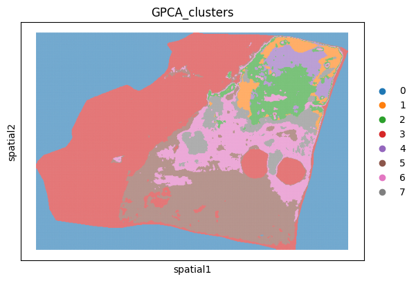
Often with Spatial Glycomics data there can be large regions outside the tissue which add noise to the data. We can use goatpy to remove pixels outside the tissue. For this example we will use clustering to identify in- vs out-of-tissue pixels, and then use gp.filter_spatialdata to remove any pixels containing noise.
[46]:
sdata = gp.graphpca_spatialdata(sdata, tables= "maldi_adata",
    library_id= 'spatial',
    n_components = 50,
    n_neighbors = 8,
    alpha = 0.5)
sdata = gp.get_kmean_clusters(sdata, tables= "maldi_adata",n_clusters = 8)
[47]:
sc.pl.spatial(sdata.tables["maldi_adata"], img_key="hires",
              color=["GPCA_clusters"], size=2, spot_size=5,
              alpha_img=0)
/var/folders/f1/3f7gj1393nb0phh8vzn910nm0000gn/T/ipykernel_40255/1680037899.py:1: FutureWarning: Use `squidpy.pl.spatial_scatter` instead.
  sc.pl.spatial(sdata.tables["maldi_adata"], img_key="hires",
[48]:
sdata = gp.filter_spatialdata(sdata, "GPCA_clusters != '0'")
  137,672 / 204,876 pixels selected (67.2%)
  Done. Result: SpatialData object
├── Images
│     └── 'he_image': DataArray[cyx] (3, 5480, 7090)
├── Points
│     └── 'centroids': DataFrame with shape: (<Delayed>, 3) (2D points)
├── Shapes
│     ├── 'annotations': GeoDataFrame shape: (24, 3) (2D shapes)
│     └── 'pixels': GeoDataFrame shape: (137672, 2) (2D shapes)
└── Tables
      └── 'maldi_adata': AnnData (137672, 121)
with coordinate systems:
    ▸ 'global', with elements:
        he_image (Images), centroids (Points), annotations (Shapes), pixels (Shapes)
[49]:
fig, axes = plt.subplots(1, 2, figsize=(20, 5))

sdata.pl.render_images("he_image")\
    .pl.render_shapes("pixels",color="1339.6")\
    .pl.show(ax=axes[0], title="Pathology Polygon-Level Annotations")

sdata.pl.render_images("he_image")\
    .pl.render_shapes("pixels",color="annotation")\
    .pl.show(ax=axes[1], title="Pathology Pixel-Level Annotations")

plt.tight_layout()
plt.show()
INFO     Rasterizing image for faster rendering.
INFO     Using 'datashader' backend with 'None' as reduction method to speed up plotting. Depending on the
         reduction method, the value range of the plot might change. Set method to 'matplotlib' to disable this
         behaviour.
INFO     Using the datashader reduction "mean". "max" will give an output very close to the matplotlib result.
INFO     Rasterizing image for faster rendering.
INFO     Using 'datashader' backend with 'None' as reduction method to speed up plotting. Depending on the
         reduction method, the value range of the plot might change. Set method to 'matplotlib' to disable this
         behaviour.
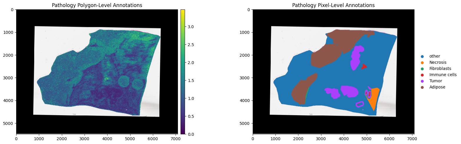
After filtering we can see the pixels outside the tissue have been removed.
Saving and Loading goatpy Ojects#
Because goatpy is built using SpatialData, any goatpy object can be stored as saved as a .zarr. This will allow for much quicker loading and exporting of data for reproducability or further downsteam analysis.
Below is an example of how to save and load data objects:
[50]:
sdata.write("./Documents/data_objects/example_data.zarr")
INFO     The Zarr backing store has been changed from None the new file path:
         /Documents/data_objects/example_data.zarr
[51]:
from spatialdata import read_zarr
sdata = read_zarr("./Documents/data_objects/example_data.zarr")
version mismatch: detected: RasterFormatV02, requested: FormatV04
Plotting and Visualising Results#
Along with the examples already displayed above, using MatPlotLib with SpatialData and scanpy there are various way to enhance and generate informative plots to support analyses. Some key implementations are demonstrated below:
Adjusting Plot Colour Palettes#
Different colour palettes are important for highlighting different types of data. Default palattes for continuous data include viridis and ```` for catagorical data. MatPlotLiB has many inbuilt cmaps which can easily be used when plotting. In the examples below, ‘jet’ and ‘Paired1’ will be used for plotting continous and catagorical data, respecitively.
[52]:
fig, axes = plt.subplots(1, 2, figsize=(10, 5))

sdata.pl.render_images("he_image") \
     .pl.render_shapes("pixels", color="MPI", cmap= "jet") \
     .pl.show(ax=axes[0])

sdata.pl.render_images("he_image") \
     .pl.render_shapes("pixels", color="GPCA_clusters", cmap = "Paired") \
     .pl.show(ax=axes[1])

plt.tight_layout()
plt.show()
INFO     Rasterizing image for faster rendering.
INFO     Using 'datashader' backend with 'None' as reduction method to speed up plotting. Depending on the
         reduction method, the value range of the plot might change. Set method to 'matplotlib' to disable this
         behaviour.
INFO     Using the datashader reduction "mean". "max" will give an output very close to the matplotlib result.
INFO     Rasterizing image for faster rendering.
INFO     Using 'datashader' backend with 'None' as reduction method to speed up plotting. Depending on the
         reduction method, the value range of the plot might change. Set method to 'matplotlib' to disable this
         behaviour.
Tutorial Session Info#
[53]:
from session_info import show
show()
[53]:
Click to view session information
-----
anndata             0.11.4
goatpy              0.1.0
matplotlib          3.10.8
napari_spatialdata  0.6.0
pandas              2.3.3
scanpy              1.11.5
session_info        v1.0.1
spatialdata         0.5.0
spatialdata_plot    0.2.12
squidpy             1.6.5
-----
Click to view modules imported as dependencies
81d243bd2c585b0f4821__mypyc NA
OpenGL                      3.1.10
PIL                         12.2.0
PyQt5                       NA
ac51d50a4f4b6d748b8c__mypyc NA
annotated_types             0.7.0
app_model                   0.5.1
appdirs                     1.4.4
appnope                     0.1.4
asciitree                   NA
asttokens                   NA
attr                        26.1.0
attrs                       26.1.0
backports                   NA
cachey                      0.2.1
certifi                     2026.02.25
charset_normalizer          3.4.7
click                       8.3.2
cloudpickle                 3.1.2
colorama                    0.4.6
comm                        0.2.3
cv2                         4.13.0
cycler                      0.12.1
cython_runtime              NA
dask                        2024.11.2
dask_image                  NA
datashader                  0.19.0
dateutil                    2.9.0.post0
debugpy                     1.8.16
decorator                   5.2.1
distributed                 2024.11.2
docrep                      0.3.2
docstring_parser            NA
dotenv                      NA
exceptiongroup              1.3.1
executing                   2.2.1
flexcache                   0.3
flexparser                  0.4
fsspec                      2026.3.0
geopandas                   1.1.3
h5py                        3.16.0
heapdict                    NA
hsluv                       5.0.4
idna                        3.11
imagecodecs                 2025.3.30
imageio                     2.37.3
importlib_metadata          NA
in_n_out                    0.2.1
ipykernel                   6.31.0
jaraco                      NA
jedi                        0.19.2
jinja2                      3.1.6
joblib                      1.5.3
jsonschema                  4.26.0
jsonschema_specifications   NA
kiwisolver                  1.5.0
lazy_loader                 0.5
legacy_api_wrap             NA
llvmlite                    0.47.0
locket                      NA
loguru                      0.7.3
magicgui                    0.10.2
markupsafe                  3.0.3
matplotlib_inline           0.2.1
matplotlib_scalebar         0.9.0
metaspace                   2.0.9
metaspace_converter         NA
more_itertools              11.0.2
mpl_toolkits                NA
msgpack                     1.1.2
multipledispatch            0.6.0
multiscale_spatial_image    2.0.3
napari                      0.7.0
napari_builtins             0.7.0
napari_plugin_engine        0.2.1
natsort                     8.4.0
networkx                    3.4.2
npe2                        0.8.2
numba                       0.65.0
numcodecs                   0.13.1
numpy                       2.2.6
ome_zarr                    NA
packaging                   26.0
parso                       0.8.6
patsy                       1.0.2
pexpect                     4.9.0
pickleshare                 0.7.5
pims                        0.7
pint                        0.24.4
pkg_resources               NA
platformdirs                4.9.6
prompt_toolkit              3.0.52
psutil                      7.0.0
psygnal                     0.15.1
ptyprocess                  0.7.0
pure_eval                   0.2.3
pyarrow                     21.0.0
pyct                        0.6.0
pydantic                    2.13.1
pydantic_core               2.46.1
pydantic_extra_types        2.11.1
pydantic_settings           2.13.1
pydev_ipython               NA
pydevconsole                NA
pydevd                      3.2.3
pydevd_file_utils           NA
pydevd_plugins              NA
pydevd_tracing              NA
pygments                    2.20.0
pyimzml                     1.5.5
pyparsing                   3.3.2
pyproj                      3.7.1
pyqtgraph                   0.14.0
pytz                        2026.1.post1
qtpy                        2.4.3
referencing                 NA
requests                    2.33.1
rich                        NA
rpds                        NA
scipy                       1.15.3
seaborn                     0.13.2
shapely                     2.1.2
sip                         NA
six                         1.17.0
skimage                     0.25.2
sklearn                     1.7.2
slicerator                  1.1.0
sopa                        2.1.11
sortedcontainers            2.4.0
spatial_image               1.2.3
stack_data                  0.6.3
statsmodels                 0.14.6
superqt                     0.8.1
tblib                       3.2.2
threadpoolctl               3.6.0
tifffile                    2025.5.10
tlz                         1.1.0
toolz                       1.1.0
tornado                     6.5.5
tqdm                        4.67.3
traitlets                   5.14.3
typing_extensions           NA
typing_inspection           NA
urllib3                     2.6.3
validators                  0.35.0
vispy                       0.16.1
vscode                      NA
wcwidth                     0.6.0
wrapt                       2.1.2
xarray                      2025.6.1
xarray_dataclass            3.0.0
xarray_schema               0.0.3
xrspatial                   0.5.3
yaml                        6.0.3
zarr                        2.18.3
zict                        3.0.0
zipp                        NA
zmq                         27.1.0
zoneinfo                    NA
-----
IPython             8.37.0
jupyter_client      8.8.0
jupyter_core        5.9.1
-----
Python 3.10.20 (main, Mar 11 2026, 17:43:48) [Clang 20.1.8 ]
macOS-26.3.1-arm64-arm-64bit
-----
Session information updated at 2026-04-17 20:06